- Research
- Open access
- Published:
Comparative study of algorithms for optimized control of industrial energy supply systems
Energy Informatics volume 3, Article number: 12 (2020)
Abstract
Both rising and more volatile energy prices are strong incentives for manufacturing companies to become more energy-efficient and flexible. A promising approach is the intelligent control of Industrial Energy Supply Systems (IESS), which provide various energy services to industrial production facilities and machines. Due to the high complexity of such systems widespread conventional control approaches often lead to suboptimal operating behavior and limited flexibility. Rising digitization in industrial production sites offers the opportunity to implement new advanced control algorithms e. g. based on Mixed Integer Linear Programming (MILP) or Deep Reinforcement Learning (DRL) to optimize the operational strategies of IESS.This paper presents a comparative study of different controllers for optimized operation strategies. For this purpose, a framework is used that allows for a standardized comparison of rule-, model- and data-based controllers by connecting them to dynamic simulation models of IESS of varying complexity. The results indicate that controllers based on DRL and MILP have a huge potential to reduce energy-related cost of up to 50% for less complex and around 6% for more complex systems. In some cases however, both algorithms still show unfavorable operating behavior in terms of non-direct costs such as temperature and switching restrictions, depending on the complexity and general conditions of the systems.
Introduction
The share of Renewable Energy Sources (RES) has increased significantly over the last two decades and further increase in the generation of RES is expected (U.S. Energy Information Administration 2019). This development is supported by the United Nations agenda for sustainable development (United Nations 2015) as well as national policies (Presse- und Informationsamt der Bundesregierung 2018). In Germany, RES have supplied 35.2% of electricity consumption in 2018 (Agora Energiewende 2019), 42.6% in 2019 (Agora Energiewende 2020) and 56.2% till June 2020 (Breitkopf 2020). The integration of RES leads to unique challenges for the existing electricity grids. In comparison to traditional energy sources, the output of many RES is highly variable. Additionally, typical conventional power plants are not flexible enough to economically compensate the unstable output of RES (Weitzel and Glock 2018). The result is that energy prices vary considerably over short periods of time (Andersen et al. 2006). Andersen et al. suggest that Demand Side Management (DSM) and Demand Response (DR) in particular can help to compensate price and power output fluctuations by adjusting demand (Andersen et al. 2006). Since the manufacturing sector is responsible for a significant share of the total energy demand in Germany (around 30%) (Deutsche Energie-Agentur 2018), it has tremendous potential to increase demand side flexibility (Sauer et al. 2019).
Energy-efficient and flexible control of industrial energy supply systems
The Industrial Energy Supply Systems (IESS) of a factory are all facilities required for the targeted conversion of final and environmental energy as well as the storage and transportation of the useful energy required for the operation of the building and the production processes (e. g. heating, cooling, electricity) (Buoro et al. 2013). To achieve or improve DSM in the manufacturing sector, operating strategies for IESS can be implemented in order to flexibilize the total energy demand of industrial sites, consisting of IESS and production machine demand. However, energy flexible and efficient IESS tend to be very complex, due to the integration of thermal storage and many interconnected systems (Panten et al. 2018). As the complexity of IESS increases, however, so do the challenges for operating facilities and systems optimally with regard to the simultaneous operation targets: (energy) costs, supply security and environmental sustainability. Due to their simple design and low implementation costs, classic rule-based methods such as two-point controllers and PID controllers are almost always used for the control and automation of IESS (Panten et al. 2018). However, for more complex, dynamic systems, a variety of challenges make it difficult to identify optimal operating strategies and translate them into manually programmable rules (Panten 2019):
-
1
IESS are typically complex energy systems with multiple inputs and multiple outputs including multivalent forms of energy.
-
2
The facilities or systems, their mode of operation and the environment often interact with each other through multivariate, non-linear relationships.
-
3
Systems with high dynamics (e. g. electrical load changes) meet systems with long time delays (e. g. thermal storage capacity of a building).
-
4
A large number of stochastic endogenous and exogenous disturbances (e. g. internal loads, weather, energy markets, production operation) have a considerable influence on the supply level or overall costs for operation (see 1).
Fig. 1 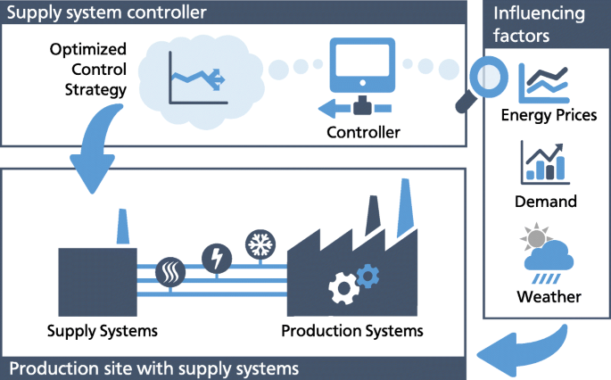
Problem description. Influencing factors such as energy prices, weather conditions and energy demand of production facilities influence the operating behavior of industrial energy supply systems. Advanced control strategies for supply systems have to take these factors into account to derive optimized control strategies
-
5
Integrated energy storages within the supply system extend the optimization complexity by a temporal flexibility dimension.
-
6
In addition to security of supply, a cost-efficient and environmentally friendly operation is required. The respective requirements and specific costs are constantly changing. An optimal operating strategy should therefore include several time-variable targets.

Due to the challenges mentioned above, the performance of conventional control processes is severely limited (Panten et al. 2018; Atabay 2017). Accordingly, there is potential for considerable energy and cost savings through the development of optimized operating strategies (Panten 2019). To demonstrate how future factories can utilize energy in a smart way, the ETA-Factory on the campus of the Technical University of Darmstadt was built (Abele et al. 2018). The model factory is at the same time the object of research, large-scale demonstrator and place of learning (Abele et al. 2016). The systems of the case study in this work is oriented on the supply systems at the ETA-Factory.
The presented paper is structured as follows: In the following chapter, the State of the Art of advanced control algorithms for energy supply systems as well as preliminary work is presented. Afterwards the case study for the comparative study is explained followed by a description of the presented framework and the implemented control algorithms. Within the evaluation section exemplary runs as well as a performance evaluation are discussed. The paper ends with a conclusion and outlook to future works.
State of the art
Highly efficient energy supply systems are particularly complex due to their high degree of cross-linking. As a result, widespread conventional control approaches often lead to sub-optimal operating behavior and thus unnecessarily high energy costs (Panten et al. 2018). Progressive digitization in industrial production plants increases the availability of high-quality data of energy systems. While this data is currently mainly used for transparency and forecast applications in production processes (condition monitoring, predictive maintenance), algorithms that optimize the operation of energy supply systems in factories are rarely represented so far (Schuh et al. 2017; Posselt 2016). Thus, high cost saving potentials by optimizing the operation strategy of comparable systems can be expected (Schiller et al. 2014; Panten 2019).
In this context model-based Model Predictive Control (MPC) algorithms already show promising results in smaller systems such as buildings, in particular with regard to dynamic weather forecasts (Petersen and Bundgaard 2014) and occupancy forecasts (Ma et al. 2010; Halvgaard 2014). For example, Ma et al. develop nonlinear models of an entire cooling system, consisting of a cooling tower, compression chillers and heat accumulators, and achieve an improvement in the Coefficient of Performance (COP) of 19.1% by means of a MPC approach (Ma et al. 2010). Široký et al. use weather forecasts for MPC of a building heating system and achieve energy savings of between 15% and 28% depending on system and weather conditions (Široký et al. 2011). While the method can in principle be applied to other “smart” energy systems (Halvgaard 2014) such as IESS, the accuracy of this method depends heavily on a high-quality modelling of system dynamics (Široký et al. 2011). In the field of MPC often mathematical programming is used to model and optimize energy supply systems. As depicted in (Kohne et al. 2019) mathematical model-based approaches based on mathematical programming - mainly Mixed Integer Linear Programming (MILP) - of converters exist (Voll and Bardow 2014; Steck 2014), but current research often implements energy grids as power balances e. g. (Atabay 2017; Saffari Tabalvandani et al. 2018; Buoro et al. 2013). Those approaches are not suitable for modeling complex thermal grids in production sites due to missing implementation of temperature dependencies and thermal inertia (Zahoransky and Allelein 2010).
Besides model-based approaches, also data-based algorithms such as the application of Deep Reinforcement Learning (DRL) is investigated to optimize the behavior of IESS (Panten 2019). These prove to be particularly advantageous compared to classical optimization methods when the system and the environment are very complex (Vázquez-Canteli and Nagy 2019), which is why DRL algorithms have been investigated in many physics and engineering domains (Garnier et al. 2019). DRL methods for energy supply systems, however, represent a comparatively young field of research. The methods are often based on long-established methods such as tabular Q-Learning with small, discretized state and action spaces (Yang et al. 2015; Liu and H. 2006; Sheikhi et al. 2016; Chen et al. 2018). Only a few recently published DRL methods are used, which are also suitable for large continuous state and action spaces. However, even these publications always consider special, comparatively small energy systems with very simple target functions (Bollenbacher and Rhein 2017; Mocanu et al. 2018). Panten identified a lack of application-ready solutions for large energy supply systems, consisting of diverse subsystems for electricity, heating, cooling and coupled Heating, Ventilation and Air Conditioning systems (Panten 2019). For this reason, a framework was set up in (Panten 2019) with respect to DRL approaches.
This work was then extended in (Panten et al. 2020) to include the possibility of integrating MPC-based algorithms and applying them to the same simulated systems, thus establishing a framework for the comparison between DRL-based, MPC/MILP-based and rule-based controllers. However, a detailed performance comparison of the various algorithms has not yet taken place and is the central part of this work.
Case study
In the comparative study of these three control algorithms, two IESS A and B of different size and complexity were chosen (see Fig. 2). The smaller system A contains a Combined Heat and Power (CHP) unit and a Condensing Boiler (B) as in state-of-the-art heat supply systems, extended by an Immersion Heater (IH) and a Hot Water Storage (HS) for more flexibility.

Representation of system A and B. System A consists of combined heat and power (CHP) unit, a condensing boiler (B), an immersion heater (IH) and a hot thermal energy storage (HS) providing heating, electricity and gas through the grids. System B additionally contains the cooling grid with a heat pump (HP) between cooling and heating grid, a cooling tower (CT), a compression chiller (CC) and a cold thermal energy storage (CS) (Panten 2019)
The larger system B complements system A with the typical central cooling supply, additionally consisting of a Compression Chiller (CC), a Cooling Tower (CT) and a Cold Water Storage (CS). To activate the CC, it’s warm side has to be cooled by the CT. Moreover, to model progressive interlinked IESS, a Heat Pump (HP) between heating and cooling grid as added.
Further, the case study is based on energy demand data of a real production site of a project partner including heating, cooling and electricity demand (peak demands are around 300 kW, 100 kW and 250 kW respectively). Moreover, weather data (obtained from Deutscher Wetterdienst) and variable energy market data (day ahead prices, obtained from a local energy provider) is integrated. The market price for gas and electricity is assumed as real time pricing model for the algorithms and it is supplemented with taxes and maximum power charges based on German legislation. Thus, the factory can be regarded as flexible consumer and producer (prosumer) within a microgrid. The objective is to optimize the control of the supply systems in order to meet the forecasted/given energy demand in the most cost effective way.
Framework
The framework used in this work is based on the one developed by Panten in (Panten 2019). The basic structure is depicted in Fig. 3 and corresponds to the structure of a Reinforcement Learning (RL) approach as presented by Sutton and Barto in (Sutton and Barto 2018). RL is learning how to match system states St to actions At in order to maximize a scalar reward signal Rt. This is done by trial and error to identify which actions bring the highest immediate and subsequent rewards (Sutton 1992). The acting unit that makes decisions and interacts with a system is called agent in the RL context, the system with which the agent interacts is commonly referred to as an environment. In Fig. 3, the left side represents the agent side of the framework. In this work, this is where the different control algorithms are implemented. The right side in Fig. 3 represents the environment side of the framework, which is where the interactive simulations of the IESS are implemented. The control algorithms calculate set points for the individual systems of the IESS. These control signals are then converted into actuating signals and forwarded to the individual components of the simulation model.

Framework. The different algorithms are represented by the multiple layers on the left side, whereas the multiple layers on the right side represent the possibility to interact with various environments, as described in the section Case Study (Panten et al. 2020)
The implementation of the framework is based on open source toolkits provided by the non-profit research organization OpenAI (Brockman 2015). OpenAI offers the Gym toolkit for the comparison of different DRL algorithms (Brockman 2016), which is used as a basis for the environment side of the framework. The agent side is based on the Stable Baselines, a set of improved implementations of RL algorithms itself based on the OpenAI Baselines (Dhariwal et al. 2017). It consists of freely available, simplified and uniform implementations of the most important DRL algorithms (Hill et al. 2018). Since the structure of the algorithms, environments and the interface connecting them is object-oriented and standardized, further algorithms and environments can be implemented without changes to the architecture of the framework.
The environments are adapted so that weather, load and price data can be imported. The simulation models of the systems of the case study can be integrated as a Functional Mock-up Unit (FMU) model via an interface that is implemented in the framework using the open source library FMPy (Dassault Systèmes 2018). The FMU models are created using the modeling language Modelica for which a library has been developed in (Panten 2019) with which the dynamic simulation models of energy systems for the case study in this work were created. The library contains models of typical production plants of the metal processing industry and common systems of building and supply engineering.
Regarding the control algorithms, conventional 2-point controllers (rule-based) were already implemented in (Panten 2019) and finally also mathematical control algorithms in (Panten et al. 2020), based on the work of Kohne et al. (Kohne et al. 2019). All control algorithms investigated in this work are depicted in Figure 4 and described in the following sections.

Control algorithms. Within the framework, different algorithms (rule-based, MILP-based, DRL-based) are tested for the control of environments. The environments are simulations of the industrial energy supply systems to be controlled
Rule-based control algorithm
Since 2-point controllers are currently one of the most used algorithms for the control and automation of supply systems (Perera et al. 2014), they provide a suitable baseline to compare the performance of DRL-based and MPC-based controllers against. The conventional controller considered in this paper activates or deactivates the respective energy converters based on the temperatures in the top (t) and bottom (b) location of the HS or CS as depicted in Fig. 2. The switch-on and switch-off rules for the individual converter are shown in Table 1. The order in which the converters are switched on is determined in advance, based on the expected average cost efficiency of the converters. The energy converters can either be switched off or switched to maximum power. Intermediate stages are not possible with this controller.
MILP-based control algorithm
The model-based control algorithm in this work is implemented with MILP models as an MPC approach based on the work of Kohne et al. (Kohne et al. 2019). During the course of this work, it is extended, adapted and standardized. The integrated MILP library consists of different energy converters and storages so that different environments can be modelled efficiently. The energy converters modeled in the MILP library are designed by modular linear equations defining inputs (gas, electricity) and outputs (electricity, heating, cooling) while energy storages are modeled as stratification storages which define the thermal grids for heating and cooling of the production processes. Moreover, this approach is able to abstract thermal dependencies and thermal inertia based on (Kohne et al. 2019; Weber et al. 2018). In order to realize the MILP library with modular components, the Python-based, open-source optimization modeling language Pyomo is used (Hart 2017). This library enables the python tool to define abstract classes of different components. These abstract models can then be integrated into overall mathematical models and individually initialized for every environment. As in all MPC and especially MILP approaches, the model represents a simplified image of the real system with the possibility to predict future system states (Halvgaard 2014).
Besidesthe integration of the MILP library, the overall model objective function is extended by further components. The objective cost function, shown in Equation 1 contains next to costs for gas \(\mathrm {c}^{\text {gas}}_{t}\) and electricity \(\mathrm {c}^{\text {el}}_{t}\) also taxes on procured energy taxgas/ taxel as well as charges for peak loads cpower. Additionally, non-direct cost for switching \(\mathrm {c}^{\text {switch}}_{t,i}\) are added. As not every optimization run might result in feasible solutions due to grid constraints, infinite sinks and sources are modeled to ensure system stability of the optimization process. These virtual energy sinks and sources are then targeted by high non-direct cost csink/source in the overall objective function:
For the scheme of continuously controlling an environment, the mathematical model initially needs to be parameterized (nominal power or capacity of components, import of external forecast values for weather, load and energy price data). Also settings specific to the task (e. g. forecast horizon, time step size/sampling time) and specific to the solving algorithm must be chosen and have a significant impact on the performance (Table 2). In this work, a Branch and Cut algorithm of the commercial solver CPLEX from IBM (IBM 2017) is used as solving algorithm. The solver CPLEX can be parameterized by setting maximum calculation time and the minimum optimality gap of the solution.
By then solving the mathematical optimization problem, control signals are optimally calculated for all components as control signal trajectory within a determined forecast horizon (Figure 4). Then, the first control signals of each component is given to the environment as actions for the specific time step t. The environment is affected the actions and returns the new states and predictions back to the agent side of the framework (Fig. 4). The basic idea is to calculate the optimal variables in a time-discrete, dynamic model at each time step depending on the anticipated future behavior of the system integrating predictions of system states (Perera et al. 2014).
This procedure continues in a loop where the model is repeatedly reparametrized after each time step by taking into account the current supply system state and external forecast values (Fig. 4). Since the forecast horizon stays the same and is extended into the future every time step, this procedure is also referred to as Receding Horizon Control (RHC) (Institute for Systems Theory and Automatic Control 2020; Dong and Lam 2014). In order to optimize calculation time in the RHC optimization, Pyomo offers the opportunity to update necessary information like new predictions into the mathematical model. Thus, a standardized function for updating the model is integrated into the framework so that it does not have to be set for each time step.
DRL-based control algorithm
The Proximal Policy Optimization (PPO) algorithm (Schulman et al. 2017) has proven to be a particularly stable and reliable method among the actor-critic DRL algorithms and therefore, PPO was chosen among the algorithms available in the Stable Baselines (Dhariwal et al. 2017) to represent the DRL approach in this work.
The PPO algorithm actively limits the change to the policy when calculating the gradients. The policy π(At|St,θ) maps system states (St) to Actions (At) according to the current parameters θ of a neural net (the “actor”), which, together with the parameters of another neural net (the “critic”) ω, are updated during the training process. The aim is to achieve the greatest possible improvement step on the basis of the currently available data without compromising the stability of the training process through too large updates. For this, the algorithm carries out the following steps (Panten 2019):
-
1
Based on the current policy π(At|St,θ) divided into Nenvs instances of the environment, a total of Nsteps interaction steps are carried out and thus state, action, reward sequences are generated. Each instance is the same simulation run in parallel to collect more data in a shorter period of time.
-
2
On the basis of the sequences, Returns Gt and Advantage values \(\hat {A}_{t}\) are calculated. Returns are aggregated, discounted rewards, whereas the Advantage values indicate the relative advantage for the chosen actions compared to the expected baseline.
-
3
For Nepochs optimization runs the same Nsteps experience sequences are mixed and divided into Nmb mini-batches.
-
4
The update of the parameters θ,ω is performed by the Adam optimizer (Kingma and Ba 2014) with the learning rate α and the experience sequences of the mini-batches based on the target function to be maximized \(L_{t}\left (\boldsymbol {\theta }, \boldsymbol {w}, S_{t}, \hat {A}_{t}\right)\).
-
5
Steps 1-4 are repeated \(\mathrm {N^{updates}}=\frac {\mathrm {N^{total}}}{\mathrm {N^{steps}}}\) times until a total of Ntotal time steps have been completed.
For a detailed description of the PPO algorithm we refer to (Schulman et al. 2017; Hill et al. 2018; Panten 2019).
The training behavior is fundamentally influenced by the given cost function, which passes a scalar reward value (Rt) to the DRL algorithm depending on the system state (see Fig. 3). In this context, costs are interpreted as negative rewards. The cost function is designed as a sum of weighted terms as shown in equation 2 (Panten 2019).
Here, \(R_{t}^{\text {limits}}\) are rewards for evaluating and limiting the state space (e.g. temperatures, electrical peak load), \(R_{t}^{\text {switches}}\) rewards for reducing the frequency with which systems are switched on, \(R_{t}^{\text {costs}}\) rewards due to real expenses (e. g. energy costs, taxes) and \(R_{t}^{\text {others}}\) additional rewards to influence the learned control strategy (e. g. punishment term at simulation abort). The hyperparameters glimits,gswitches,gcosts,gothers are used to weight the individual terms meaningfully. To ensure that the temperature limits of the systems in the case study are not exceeded, for example, a relatively high value is chosen for glimits. Furthermore, since the normalization of the inputs and outputs of the neural net has a significant influence on the learning speed or convergence behavior (Goodfellow et al. 2016), the continuous state variables and reward values given to the DRL-algorithm are always normalized to the interval [0,1]. The Multi Layer Perceptron (MLP) (see (Goodfellow et al. 2016)) topology was used for the neural network. The PPO algorithm was used with a discrete action space, allowing for the selection of predefined set points for the individual supply systems. The hyperparameters for the algorithm itself are shown in Table 3.
The training process was complete after around 1000 episodes (one episode being three randomly chosen days divided by a step size of 180 seconds) and took around 12 hours on an Intel Core i7-8550U Processor without graphics card utilization for the training of the DRL-algorithms.
Performance evaluation
The presented framework with its algorithms is evaluated within a comparative study for both systems as described in the case study. The characteristics of each control algorithm are shown by displaying two exemplary test runs, one for each system. Subsequently, the performance of the individual algorithms is statistically evaluated for 100 randomly selected days. In the following, the former described specific MILP- and DRL-based control algorithms are referred to just as MILP and DRL respectively.
Exemplary test runs
With each control algorithm - Conventional/rule-based, MILP-based and DRL-based - test episodes of a seven day duration and a three minute sampling time were simulated on each system in order to analyze specific behavior of the different control algorithms. The sampling time describes the length of one time step. A first obvious difference between the control algorithms is the initial parameterization. While the conventional controller is parameterized just by setting temperature restrictions and a ranking for the energy converters (compare Table 1), the MILP model has to be set up with fixed parameters such as nominal power as well as soft parameters like thermal delay. The parameterization of the DRL algorithm is based on hyper parameter variations as carried out in (Panten 2019) (e. g. learning rate neural network topology).
In system A, the set points for CHP, B and IH have to be chosen by the control algorithms, in effect choosing to either use gas or electricity for heating supply. Moreover, electricity can be produced by using the CHP unit. In Fig. 5 a test episode of system A is shown, displaying a selection of input data, the set points chosen by each algorithm and the resulting electrical grid power as well as temperatures of the HS. The demand curves of the first subplot show a two shift production plan on week days without any production on weekends. Within a production shift, the demands for electric power is up to 250 kW and 310 kW for heating, respectively. Moreover, the electricity prices at the beginning of the episode are relatively high up to 0.16 €/kWh.

Exemplary test run of system A with an episode duration of seven days and a sampling time of three minutes. Subplot 1 shows input parameters as electricity and heating demand of the production system as well es electricity prices. Subplots 2-4 show the resulting actions of the control algorithms and subplots 5 and 6 contain the electric power demand to the grid and the temperature of the HS
Compared to the conventional controller with an evenly behavior within the week days, the MILP controller heats up the heating grid up to the allowed 90 ∘C within the first two days. The more constant use of the CHP unit leads a reduced peak load of around 10 kW and savings electricity cost at high prices. Moreover, in this episode, the DRL-algorithm cannot meet the lower temperature restrictions at all times.
In system B a cooling demand is added which can be supplied by the CC or CT while the efficiency of the CT is highly dependent on the outside temperature. Moreover, the optimized control strategy can be chosen more flexibility by utilizing the HP in order to supply both, heating and cooling. Figure 6 displays a test episode for system B of the same scenario as shown before. Here, the cooling demand is up to 50 kW.

Exemplary test run of system B with an episode duration of seven days and a sampling time of three minutes. Subplot 1 shows input parameters as electricity and heating demand of the production system as well es electricity prices. Subplots 2-4 show the resulting actions of the control algorithms and subplots 5 and 6 contain the electric power demand to the grid and the temperature of the HS and CS
The action heat maps also show a more volatile behavior of the DRL- and MILP-based algorithms compared to the conventional controller. This way, the MILP-algorithm can reduce peak loads by around 10 kW, the DRL even around 100 kW. Nevertheless, the DRL-algorithm shows an abnormal use of the CC. In the simulation model, the CC cannot be activated without the CT. Thus, the volatile switching of the CC within the DRL actions do not result in a use of the CC. In the training process, the DRL-algorithm must have learned that those kind of actions do not lead to lower rewards. Although it would not have led to destructive system behaviour in this case, it is a good example of the problem of the lack of explainability of the actions generated by DRL methods.
Cost evaluation
For the overall evaluation, all controllers were operated on the same 100 episodes, each with an duration of 24 hours and a sampling time of 180 seconds, randomly chosen from the year 2018, so that summer as well as winter days with different environmental conditions (temperature, humidity) were simulated.
Figure 7 shows the cost-related results for system A. In particular, the energy-related costs (top right) show revenue opportunities through the use of the MILP or DRL controller. Here, the MILP controller achieves cost savings of about 13%, the DRL controller even more than 50%. Thus, a high potential of energy cost reduction through the use of algorithms that can include a multitude of current data as well as forecasts in their decisions is shown. Besides direct cost of energy procurement, also non-direct costs such as switching costs or penalty costs for temperature violations have to be taken into account. In this case, the overall revenue potential (top left) are still up to 8% for the MILP controller and 33% for DRL respectively.

Distribution and mean value of overall and specific cost per episode for system A. Cost in this case are interpreted as negative rewards, thus increasing performance is indicated by higher values. Black: Conventional controller, Blue: DRL controller, Green: MILP controller
For the more complex System B, the potential for reducing energy-related costs is shown to be 3% (MILP) and 6% (DRL) (Fig. 8). Despite the increased complexity, the algorithms are also able to take into account the large number of possible influences and thus reduce energy costs. However, the complexity also results in an unconventional control behavior that increases the non-direct costs. This results in cost increases of 50% compared to the conventional controller.

Distribution and mean value of overall and specific cost per episode for system B. Cost in this case are interpreted as negative rewards, thus increasing performance is indicated by higher values. Black: Conventional controller, Blue: DRL controller, Green: MILP controller
Although both, MILP and DRL can reduce direct cost for energy procurement, it is noticeable that the DRL controller incurs high penalty costs for temperature restrictions and the MILP controller incurs high penalty costs for start-up and shut-down behavior. Since the DRL approach as a data-based method it is not bound to fixed restrictions and temperature requirements in particular cannot always be adhered to without a fall-back level. With the MILP approach, which optimizes over a longer period of time, penalty costs for this optimization period can be priced in. However, the receding horizon approach (only the first time step is executed) leads to a tendency for start-up and shut-down behavior in the first time step of each optimization.
Energetic evaluation
Additionally to potential cost savings, possible energy and CO2 savings have to be considered. Assuming CO2 emission factors for the German energy market of 0.537 kg/kWh for electricity and 0.202 kg/kWh for gas, the results of the different controllers vary considerably. For system A (Fig. 9) the DRL approach can reduce both energy consumption and CO2 emissions, but for system B (Fig. 10) it shows worse results than the conventional controller. In most cases, the MILP approach provides similar results to the conventional controller. The current assumption of static CO2 values of energy sources leads to a low correlation between electricity price and specific CO2 emissions, especially in the case of electricity. Conventional operating strategies based on gas-fired technologies (CHP is operated at full load if possible) therefore show good results for CO2 emissions. Innovative algorithms could take advantage of this correlation by using time-variable CO2 factors for electricity, which would also correlate more strongly with the electricity price due to the fluctuation of renewable energies.

Distribution and mean value of energy consumption and CO2 emissions per episode for system A. Black: Conventional controller, Blue: DRL controller, Green: MILP controller

Distribution and mean value of energy consumption and CO2 emissions per episode for system A. Black: Conventional controller, Blue: DRL controller, Green: MILP controller
Holistic discussion
The overall results show on the one side that the DRL and the MILP controller have a huge potential to reduce energy-related cost of IESS. The capability of taking different environmental data into account enables the controllers to anticipate, for example, rising electricity prices or weather changes in order to adapt their respective operating strategies accordingly. On the other side, both algorithms show unfavorable behavior in terms of non-direct cost such as temperature restrictions and switching cost depending on the complexity and general conditions of the systems, which can lead to technically unfavorable actions. Table 4 shows various cost items and energy consumption of DRL and MILP controllers in relation to the conventional controller.
Overall, these results confirm that the approaches are particularly applicable to subsystems in IESS and usually have a high potential for reducing energy-related costs. However, the higher the complexity of the systems, the more difficult it is to implement the algorithms precisely and thus to achieve general practicability. The practicability of the operational optimization of IESS depends on a number of factors that must be considered individually for each IESS. The effort and cost for implementing those advanced algorithms correlates with the necessity of modelling or creating simulations/mathematical models, training or testing the algorithms on a powerful computer, commissioning and purchasing any software licences. In order to justify the effort of the installation, the controllers have to prove to be as robust as classical control methods such as rule based algorithms. For this reason, the procedures cannot currently be applied to systems of any complexity. The following aspects should therefore be considered in detail:
-
The availability of high-quality scenario data (e. g. load profiles, weather) is necessary for the application of advanced algorithms. If insufficient or incorrect data is used for the training scenarios or the parameterization of the mathematical models, a suboptimal operating behavior may occur, which compromises the expected cost savings.
-
The more complex and different the energy systems of the considered system with multiple target variables are, the more difficult it is to parameterize the methods. In the case of the MILP controller this refers to the parameterization of the linear, mathematical model; in the case of the DRL it refers to learning an advantageous strategy. For this reason, it is advisable to first optimize subsystems of the energy supply system that are as decoupled as possible, such as the heat or cold supply with associated systems.
-
The consideration of cross-sectional technologies reduces the modeling effort, since recurring and sufficiently known as well as evaluated models can be used in the simulation library/optimization library. In this case, the parameterization of the interconnected systems can be carried out efficiently. If exotic technologies or very individual systems are considered, the creation of simulation models / mathematical models can be very complex.
Conclusion
This paper presents a comparative study of different control algorithms based on different approaches for optimized operation strategies of IESS. For that, a training framework, consisting of a simulation library and optimization framework with different control algorithms was adapted and evaluated. The framework allows a standardized comparison of rule-, model- and data-based controllers by connecting them to dynamic simulation models of IESS of varying complexity. In this way different operating strategies and behaviors can be evaluated and potentially cost and energy savings are identified. Within the performance evaluation three controllers - conventional/rule-based, MILP-based and DRL-based - are applied on two supply systems, the heat supply system A, and a second system B, which supplements system A by a cooling grid.
The overall results show on the one hand that the DRL-based and the MILP-based controller have a huge potential to reduce energy-related cost of IESS up to 50% in less and around 6% more complex supply systems. The capability of taking different environmental data into account enables the controllers to anticipate, for example, rising electricity prices or weather changes in order to adapt their respective operating strategies accordingly. On the other hand, both algorithms show unfavorable behavior in terms of non-direct cost such as temperature restrictions and switching cost depending on the complexity and general conditions of the systems, which can lead to technically unfavorable actions.
Both presented advanced control algorithms - MILP-based and DRL-based - show different strengths and weaknesses in the comparative study. Thus, in future work, the now existing framework can be used to conduct further research on the single algorithms, but also on combination of both approaches in order to dispel each weaknesses. Furthermore, ongoing research is focusing on objective comparability key performance indicators between data-based and model-based approaches. Thus, dependencies for non-direct cost behaviour can be further analyzed. Lastly, the presented framework will be connected to the physical systems at the ETA-Factory to test algorithms in a standardized framework on real supply systems.
Availability of data and materials
The data sets analyzed during the current study are available from the corresponding author on reasonable request.
Abbreviations
- RES:
-
Renewable Energy Sources
- DSM:
-
Demand Side Management
- DR:
-
Demand Response
- IESS:
-
Industrial Energy Supply Systems
- MPC:
-
Model Predictive Control
- MILP:
-
Mixed Integer Linear Programming
- DRL:
-
Deep Reinforcement Learning
- RL:
-
Reinforcement Learning
- FMU:
-
Functional Mock-up Unit
- RHC:
-
Receding Horizon Control
- PPO:
-
Proximal Policy Optimization
- COP:
-
Coefficient of Performance
- CS:
-
Cold Water Storage
- HS:
-
Hot Water Storage
- CHP:
-
Combined Heat and Power
- B:
-
Condensing Boiler
- IH:
-
Immersion Heater
- CC:
-
Compression Chiller
- CT:
-
Cooling Tower
- HP:
-
Heat Pump
- MLP:
-
Multi Layer Perceptron.
References
Abele, E, Bauerdick CJH, Strobel N, Panten N (2016) ETA Learning Factory: A Holistic Concept for Teaching Energy Efficiency in Production.
Abele, E, Schneider J, Beck M, Andreas M (2018) ETA - die Modell-Fabrik, Energieeffizienz weiter gedacht. https://tubiblio.ulb.tu-darmstadt.de/105750/.
Agora Energiewende (2019) Die Energiewende im Stromsektor: Stand der Dinge 2018: Rückblick auf die wesentlichen Entwicklungen sowie Ausblick auf 2019.
Agora Energiewende (2020) Die Energiewende im Stromsektor: Stand der Dinge 2019: Rückblick auf die wesentlichen Entwicklungen sowie Ausblick auf 2020.
Andersen, FM, Jensen SG, Larsen HV, Meibom P, Togeby M (2006) Analyses of Demand Response in Denmark.
Atabay, D (2017) An Open-Source Model for Optimal Design and Operation of Industrial Energy Systems.
Bollenbacher, J, Rhein B (2017) Optimal configuration and control strategy in a multi-carrier-energy system using reinforcement learning methods In: 2017 International Energy and Sustainability Conference (IESC), 1–6.
Breitkopf, A (2020) Monatlicher Anteil erneuerbarer Energien an der Stromerzeugung in Deutschland bis 2020 | Statista.
Brockman, G (2015) Introducing OpenAI. https://openai.com/blog/introducing-openai/.
Brockman, G (2016) OpenAI Gym. https://arxiv.org/pdf/1606.01540.
Buoro, D, Casisi M, Nardi A, Pinamonti P, Reini M (2013) Multicriteria Optimization of a Distributed Energy Supply System for an Industrial Area.
Chen, Y, Norford LK, Samuelson HW, Malkawi A (2018) Optimal Control of HVAC and Window Systems for Natural Ventilation Through Reinforcement Learning.
Dassault Systèmes (2018) FMPy. https://github.com/CATIA-Systems/FMPy.
Deutsche Energie-Agentur (2018) dena-Leitstudie Integrierte Energiewende: Impulse für die Gestaltung des Energiesystems bis 2050.
Dhariwal, P, Hesse C, Klimov O, Nichols A, Plappert M, Radford A. e. a. (2017) OpenAI Baselines. https://github.com/openai/baselines.
Dong, B, Lam KP (2014) A Real-Time Model Predictive Control for Building Heating and Cooling Systems Based on the Occupancy Behavior Pattern Detection and Local Weather Forecasting.
Garnier, P, Viquerat J, Rabault J, Larcher A, Kuhnle A, Hachem E (2019) https://arxiv.org/pdf/1908.04127.
Goodfellow, I, Bengio Y, Courville A (2016) Deep Learning. MIT Press.
Halvgaard, R (2014) Model Predictive Control for Smart Energy Systems.
Hart, WE (2017) Pyomo - Optimization Modeling in Python. Springer.
Hill, A, Raffin A, Ernestus M, Gleave A, Kanervisto A, Traore R, Dhariwal P, Hesse C, Klimov O, Nichol A, Plappert M, Radford A, Schulman J, Sidor S, Wu Y (2018) Stable Baselines. https://github.com/hill-a/stable-baselines.
IBM (2017) ILOG CPLEX 12.7 User’s Manual (IBM ILOG CPLEX Division, IBM, Incline Village, NV).
Institute for Systems Theory and Automatic Control (2020) Model Predictive Control. https://www.ist.uni-stuttgart.de/research/topics/mpc.
Kingma, DP, Ba J (2014) Adam: A Method for Stochastic Optimization. https://arxiv.org/pdf/1412.6980.
Kohne, T, Becker PA, Weber T, Panten N, Abele E (2019) Modeling approach for thermal dependencies in complex industrial energy supply system.
Liu, S, H. GP (2006) Experimental Analysis of Simulated Reinforcement Learning Control for Active and Passive Building Thermal Storage Inventory. Part 2: Results and Analysis.
Ma, Y, Borrelli F, Hencey B, Coffey B, Haves P (2010) Model Predictive Control for the Operation of Building Cooling Systems.
Mocanu, Mocanu, Nguyen, Liotta, Webber, Gibescu, Slootweg (2018) On-Line Building Energy Optimization Using Deep Reinforcement Learning.
Panten, N (2019) Deep Reinforcement Learning zur Betriebsoptimierung hybrider industrieller Energienetze. PhD Thesis, Technical University of Darmstadt.
Panten, N, Ranzau H, Kohne T, Moog D, Abele E, Weigold M (2020) Simulation und Optimierung kombiniert. https://tubiblio.ulb.tu-darmstadt.de/119472/.
Panten, N, Strobel N, Sossenheimer J, Abele E (2018) Framework for an Energy Efficient and Flexible Automation Strategy and Control Optimization Approach of Supply Systems within a Thermally-Linked Factory.
Perera, DWU, Pfeiffer CF, Skeie N-O (2014) Control of Temperature and Energy Consumption in Buildings - a Review.
Petersen, S, Bundgaard KW (2014) The Effect of Weather Forecast Uncertainty on a Predictive Control Concept for Building Systems Operation.
Posselt, G (2016) Towards Energy Transparent Factories.
Presse- und Informationsamt der Bundesregierung (2018) Deutsche Nachhaltigkeitsstrategie: Aktualisierung 2018.
Saffari Tabalvandani, M, Gracia Cuesta Ad, Fernàndez Camon C, Belusko D, Boer M, Cabeza LF (2018) Optimized Demand Side Management (DSM) of Peak Electricity Demand by Coupling Low Temperature Thermal Energy Storage (TES) and Solar PV.
Sauer, A, Abele E, Buhl HU (2019) Energieflexibilität in der deutschen Industrie: Ergebnisse aus dem Kopernikus-Projekt - Synchronisierte und energieadaptive Produktionstechnik zur flexiblen Ausrichtung von Industrieprozessen auf eine fluktuierende Energieversorgung (SynErgie). Fraunhofer Verlag.
Schiller, H, Mai R, Haendel C (2014) Chancen der Energetischen Inspektion für Gesetzgeber, Anlagenbetreiber und die Branche: Abschlussbericht zum Forschungsvorhaben.
Schuh, G, Anderl R, Gausemeier J, Hompel M. t., Wahlster W (2017) Industrie 4.0 Maturity Index - Managing the Digital Transformation of Companies.
Schulman, J, Wolski F, Dhariwal P, Radford A, Klimov O (2017) Proximal Policy Optimization Algorithms. https://arxiv.org/pdf/1707.06347.
Sheikhi, Rayati, Ranjbar (2016) Demand Side Management for a Residential Customer in Multi Energy systems.
Široký, J, Oldewurtel F, Cigler J, Prívara S (2011) Experimental Analysis of Model Predictive Control for an Energy Efficient Building Heating System.
Steck, MHE (2014) Entwicklung und Bewertung von Algorithmen zur Einsatzplanerstellung virtueller Kraftwerke.
Sutton, RS (1992) Reinforcement Learning.. Springer.
Sutton, RS, Barto AG (2018) Reinforcement Learning: An Introduction. MIT Press.
U.S. Energy Information Administration (2019) Annual Energy Outlook 2019 with projections to 2050, Washington.
United Nations (2015) Transforming our World: The 2030 Agenda for Sustainable Development: Sustainable Development Goals.
Vázquez-Canteli, JR, Nagy Z (2019) Reinforcement Learning for Demand Response: A Review of Algorithms and Modeling Techniques.
Voll, P, Bardow A (2014) Automated optimization based synthesis of distributed energy supply systems. PhD thesis.
Weber, T, Strobel N, Kohne T, Wolber J, Abele E (2018) Realistic Modeling of a Combined Heat and Power Plant in the Context of Mixed Integer Linear Programming.
Weitzel, T, Glock CH (2018) Energy Management for Stationary Electric Energy Storage Systems: A Systematic Literature Review.
Yang, L, Nagy Z, Goffin P, Schlueter A (2015) Reinforcement Learning for Optimal Control of Low Exergy Buildings.
Zahoransky, R, Allelein H-J (2010) Energietechnik: Systeme zur Energieumwandlung ; Kompaktwissen für Studium und Beruf.
Acknowledgements
The authors gratefully acknowledge the financial support of the Project Phi-Factory by the Federal Ministry of Economic Affairs and Energy (BMWi) and the project supervision by the Projektträger Jülich (PtJ).
About this supplement
This article has been published as part of Energy Informatics Volume 3 Supplement 1, 2020: Proceedings of the 9th DACH+ Conference on Energy Informatics. The full contents of the supplement are available online at https://energyinformatics.springeropen.com/articles/supplements/volume-3-supplement-1.
Funding
Publication costs were covered by the DACH+ Energy Informatics Conference Organizers, supported by the Swiss Federal Office of Energy.
Author information
Authors and Affiliations
Contributions
T. Kohne and H. Ranzau significantly conceptualized, implemented and validated the presented work by extending the framework and initializing the comparative study. N. Panten gave important input and provided the basis for the simulation model and the framework with his Phd thesis. M. Weigold supported the presented work by supervision and funding acquisition. All authors provided feedback and helped shape the research, analysis, and manuscript.
Corresponding author
Ethics declarations
Competing interests
The authors declare that they have no competing interests.
Additional information
Publisher’s Note
Springer Nature remains neutral with regard to jurisdictional claims in published maps and institutional affiliations.
Rights and permissions
Open Access This article is licensed under a Creative Commons Attribution 4.0 International License, which permits use, sharing, adaptation, distribution and reproduction in any medium or format, as long as you give appropriate credit to the original author(s) and the source, provide a link to the Creative Commons licence, and indicate if changes were made. The images or other third party material in this article are included in the article’s Creative Commons licence, unless indicated otherwise in a credit line to the material. If material is not included in the article’s Creative Commons licence and your intended use is not permitted by statutory regulation or exceeds the permitted use, you will need to obtain permission directly from the copyright holder. To view a copy of this licence, visit http://creativecommons.org/licenses/by/4.0/.
About this article

Cite this article
Kohne, T., Ranzau, H., Panten, N. et al. Comparative study of algorithms for optimized control of industrial energy supply systems. Energy Inform 3 (Suppl 1), 12 (2020). https://doi.org/10.1186/s42162-020-00115-7
Published:
DOI: https://doi.org/10.1186/s42162-020-00115-7