- Research
- Open access
- Published:
A comprehensive study on battery electric modeling approaches based on machine learning
Energy Informatics volume 4, Article number: 17 (2021)
Abstract
Battery electric modeling is a central aspect to improve the battery development process as well as to monitor battery system behavior. Besides conventional physical models, machine learning methods show great potential to learn this task using in-vehicle data. However, the performance of data-driven approaches differs significantly depending on their application and utilized data set. Hence, a comparison among these methods is required beforehand to select the optimal candidate for a given task.In this work, we address this problem and evaluate the strengths and weaknesses of a wide range of possible machine learning approaches for battery electric modeling. In a comprehensive study, various conventional regression methods and neural networks are analyzed. Each method is trained and optimized based on a large and qualitative data set of automotive driving profiles. In order to account for the influence of time-dependent battery processes, both low pass filters and sliding window approaches are investigated.As a result, neural networks are found to be superior compared to conventional regression methods in terms of accuracy and model complexity. In particular, Feedforward and Convolutional Neural Networks provide the smallest average error deviations of around 0.16%, which corresponds to an RMSE of 5.57mV on battery cell level. With automotive time series data as focus, neural networks additionally benefit from their ability to learn continuously. This key capability keeps the battery models updated at low computational costs and accounts for changing electrical behavior as the battery ages during operation.
Introduction
To reduce global greenhouse gas emissions and to enhance the air quality in densely populated regions, more and more automotive manufacturers are switching to electrifying their fleets. In 2019, the global electric vehicle (EV) market grew by more than 40% compared to 2018 (International Energy Agency (IEA) 2021). Additionally, leading automotive companies such as Volkswagen are investing heavily in the expansion of the battery value chain in the coming years (Volkswagen AG 2021).
In order to transform the automotive sector economically and successfully, the cost of battery cell manufacturing and analytics must be drastically reduced. A significant cost driver in the acceleration of the EV development process is the modeling of battery cells. The idea behind modeling is the creation of a digital twin of the battery. The digital twin can in turn be used to perform analyses in simulations without having to investigate real battery cells. This step saves both manufacturing capacities and, more importantly, the very limited test facilities.
In the literature, established physical models, such as the equivalent circuit model (ECM) (Zhang et al. 2017), are widely used in the field of battery modeling. The ECM is a theoretical circuit that retains all the electrical characteristics of a battery by using only passive electrical components. The passive electrical components are typically parameterized by laboratory measurements, such as electrochemical impedance spectroscopy (EIS) at different temperatures and states of charge (SOCs) (Choi et al. 2020). However, the estimated model parameters are only valid for a given state of health (SOH) of the battery. During the battery lifetime, the SOH degrades due to a variety of complex aging mechanisms. The main drivers are the high SOC during storage, as well as the electrical, thermal, and mechanical stress on the battery (Waldmann et al. 2014). During EV utilization, the electro-thermal load on the battery is highly individual and so is the aging. As a result, the ECM needs to be recalibrated during operation. Considering costly laboratory EIS measurements and limited test facilities, this procedure is not feasible for economical driven large electrified fleets.
Data-driven models offer a solution to overcome extensive laboratory experiments. According to a comprehensive review by Wu et al. (2020), battery modeling based on machine learning (ML) is steadily gaining importance in future applications due to their low expert knowledge and high flexibility. The majority of ML battery analysis in literature focuses on the evaluation of pre-defined feature of interest (FOI), such as capacity fade (Severson et al. 2019) (Stanford battery data set), voltage and temperature gradients (Stroe and Schaltz 2020), or charge throughput during laboratory cycling (Li et al. 2020) (NASA battery data set). Although various ML methods are already investigated, including regression methods (Wang et al. 2020), filter-based approaches (Zhang and Lee 2011), artificial neural networks (Vidal et al. 2020), and the comparison between different ML methods (Chandran et al. 2021), the focus remains primarily on FOI analyses subjected to laboratory conditions. However, according to Xiong et al. (2018), the performance of ML algorithms highly differs in terms of their application. Moreover, You et al. (2016) and Tian et al. (2020) pointed out, that the aging characteristics and FOI during laboratory cycling are not comparable and thus not transferable to real vehicle operation.
A way to use operational data for battery analysis is the so-called system identification approach. The concept behind system identification is to learn the electro-thermal battery function from operational data, as illustrated in Fig. 1. Here, ML algorithms are capable of independently identifying correlations based on in-vehicle data (Li et al. 2019), which can be used for battery model parametrization. Thus, the cost-intensive and limited laboratory tests can be avoided. In the literature, different regression methods (Lucu et al. 2018; Andersson et al. 2020) are investigated for system identification purposes, as well as neural networks (Shen et al. 2020; Heinrich and Pruckner 2020). These methods show good performance both in terms of accuracy and applicability. A comparison of ML methods for battery electric modeling using time series operational in-vehicle data is missing in literature.

Concept of system identification approach. A digital battery model learns the electro-thermal behavior based on operational in-vehicle data
In this work, we address this problem and investigate the strengths and weaknesses of a wide range of possible ML approaches for battery electric modeling. In contrast to the commonly used laboratory procedures to parameterize battery models, we focus exclusively on automotive operational cycles. Contrasted are a variety of established ML approaches, such as regression methods and different neural network architectures. The goal is a comparative analysis of battery electric modeling based on relevant ML algorithms using a uniform time series data set.
The remainder of this paper is organized as follows: “Battery electric modeling” section introduces the used methodology, together with the data set. Afterwards, “Machine learning methods” section briefly describes the evaluated ML methods. After a short description of the hardware and evaluation metrics in “Evaluation” section, the results of our experiments are provided and discussed in “Results and discussion” section. Finally, a short conclusion is drawn in “Conclusion” section.
Battery electric modeling
The aim of the data-driven methods is to replace the physical models, such as the ECM. As shown in Fig. 2, the physical model can also be considered as a black box, whose battery-electric function outputs the voltage response U(t) for a given electrical load described by a sequence of the current I(t), temperature T(t) and the remaining battery charge Q(t) (Heinrich et al. 2021).

ML methods replace physical based ECM
The basis for learning the battery-electric function is exclusively dynamic battery data during automotive operation. For this purpose, ML methods require a large amount of data from as many different driving situations as possible (Heinrich et al. 2021). To provide a comprehensive, large, and diverse quantity of data, synthetic battery data is used. The synthetic load behavior of the battery is provided using an ECM. The ECM is parameterized in advance using laboratory experiments on an automotive 60Ah NMC battery. The parameterized ECM then simulates four different driving cycles including Worldwide harmonized Light Duty Test Cycle (WLTC) (Orliński et al. 2019) as well as comparable individual urban and interurban driving scenarios. The database comprises the required battery-electric signals (I,T,Q,U) in 100ms (10Hz) resolution during vehicle operation at random ambient temperatures between -10 ∘C to 40 ∘C. To increase diversity, the current of each driving cycle within a sequence is randomly amplified by a factor α∈[0.5,1.5] to simulate different variations in driving intensities. In addition, this process is repeated based on several battery cell aging states, resulting in a total of over 48 Mio. data points, representing 352 individual automotive discharges. Based on this uniformed data set, different ML algorithms are evaluated in terms of prediction accuracy, model complexity, speed, and computational resources.
Training, validation and testing set
The training (56%), validation (19%), and testing set (25%) are built as follows: First, one of the driving profiles is held out as a testing set, which leads to 264 discharges for training and validation and 88 for testing. For the validation set, 25% of the discharges are randomly selected from each of the remaining driving profiles and each battery cell aging state. This leads to 66 discharges in the validation set and 198 discharges in the training set.
Two additional preprocessing steps are done on the data: First, white Gaussian noise is added on I, T, and U in order to fit the synthetic battery data to real measurement inaccuracies. For the mean and standard deviation, characteristics of automotive sensors are used to obtain a data set as close as possible to the situation inside real EVs (Li et al. 2020). Therefore, the sensor inaccuracies are considered using a tolerance of cell temperature (ΔT: ±1K), voltage response (U: ±8mV), and electric current (ΔI: ±0.5% of the actual current, with a least ±10mA and at maximum ±2.5A). As the charge throughput Q is calculated by the integration of I (Coulomb-Counting), it is also affected by the noise, especially by the sensor drift. Second, all features are normalized, so that each input signal is considered equally. For normalization, the MinMaxScaler() (Pedregosa et al. 2011) scales each feature to an equal range between -1 and +1 in a linear way.
Time-dependent battery behavior
According to Klass (2015) it is important to capture the effects of a time-dependent voltage response in battery modeling. The necessary temporal information is provided by extending the input sampling in two different ways: either the input is extended by variables of the current history (CH) or by the past sequence of selected signals (sliding window approach).
The CH variables are calculated by using a low pass filter (PT-1 term) as shown in Eq. 1.
The current at time step t is denoted as It and the sampling rate Δt=0.1s is equal to the signal resolution. The time constant τ represents the time look-back and makes the PT-1 term equivalent to an exponentially weighted moving average. For the experiments, two separate CH variables are calculated by using two different time constants τ. The time constant of the first CH is set to τCH,1=1 and aims to model the fast-changing battery resistances, charge transfer procedures, and double-layer capacities occurring inside the battery cell (Zhang and Harb 2013). The time constant of the second CH is set to τCH,2=250, in order to model the slow-changing diffusion processes inside the cell (Hu et al. 2012).
However, using CH variables comes with two major drawbacks: First, finding the optimal values for τ needs to be done in advance by laboratory experiments, which are undesired. And second, the optimal τ is changing depending on the individual aging state of the battery.
As a consequence, a sliding window approach as input for the neural network models is investigated. The sliding window approach does not make use of the PT-1 term and is therefore not dependent on any time constant τ. The selected sequence length is set to SL=100 with a stride of Str=12, as illustrated in Fig. 3. Whereas the sequence length is limited by computational resources, the stride needs to be set as a trade-off: A far look-back, corresponding to a high stride, is beneficial to capture more information about the slow diffusion processes. However, the stride also needs to be kept low enough to obtain enough information in the recent history to capture the fast processes in the battery cell. The mentioned stride of 12 shows to be a good compromise between those goals. It enables the networks to observe the current signal Iseq as well as the temperature Tseq and charge Qseq of the last two minutes in a high resolution.

Sliding window approach applied to historical current signal at sample-time 1760 (green). The selected sequence length SL=100 and stride Str=12 is representing a look-back of 1200 current samples (2min)
Machine learning methods
Using the preprocessed battery signals, a wide range of ML methods are trained and evaluated with the goal of learning the electric battery behavior based on a uniform database of automotive driving cycles. The explored ML methods include classical regression methods implemented using the python library Scikit-learn (Pedregosa et al. 2011), whereas the framework of the neural network is based on Keras (Chollet and et al. 2015). Due to the different processing principles, the studied ML algorithms are divided into methods using low pass filter or the sliding window approach as temporal current information.
Methods using low pass filter variables
The ML algorithms studied with PT-1 history variables include various conventional regression methods as well as neural networks:
-
Multiple Linear Regression (MLR)
-
Support Vector Regression (SVR)
-
K-Nearest Neighbor Regression (K-NN)
-
Decision Tree
-
Random Forest
-
AdaBoost
-
Gradient Boosting Regression (GBR)
-
Feedforward Neural Networks (FFNN)
Although the discharge behavior of the battery cell is highly non-linear, especially at low SOCs, the simple and intuitive MLR model (Hastie et al. 2009) is primarily analyzed. In order to pay more attention to the non-linearity, the kernel SVR is also taken into account, which is also used for SOH estimation out of a virtual battery model inKlass (2015). In SVR, important hyperparameters are the width of the ε-insensitive zone, and C, which is a trade-off parameter between the two optimization goals in SVR: a flat model function on the one side and as few deviations as possible from the ε-tube on the other side (Smola and Schölkopf 2004).
The prediction of K-NN is based on the comparison to a large reference table of training samples (Hastie et al. 2009). Here, the important hyperparameters are the number of nearest neighbors k, which also controls the model complexity, and the metric power factor p in the Minkowski distance. Additionally, the K-D tree structure for organizing the data set is used, as this enables logarithmic query times in the number of training samples (Pedregosa et al. 2011), leading to significantly shorter validation and testing times.
The decision tree is introduced by Breiman inBreiman et al. (1984) and appears to be an interesting solution due to its simplicity and white-box nature. In decision trees, the maximum number of leaf nodes Nleaves can be adjusted in order to control the total size of a tree. However, special attention must be paid to efficiently limit the maximum number of Nleave, otherwise the tree has the possibility to memorize each individual training sample. To prevent the tree from overfitting, a minimum number of training samples in each leaf node is set to 5. Multiple decision trees can also be combined to build an ensemble, such as Random Forests (Hastie et al. 2009) or AdaBoost (Drucker 1997). Random forests use bootstrap averaging, whereas in boosting, each subsequent tree takes the performance of the previous tree into account. Although AdaBoost belongs to the category of “weak learners”, the performance improves with increasing number of leaf nodes along with negligible impact on computational effort. For comparability, both ensemble approaches use the optimized number of leaves Nleave from the decision tree experiment. In the Scikit-learn version of AdaBoost.R2, additional important hyperparameter choices are the loss function and the learning rate η. GBR (Friedman 2000) is another boosting approach, in which the histogram-based version is chosen instead of the standard GBR, due to its strong improvement in speed (Ke et al. 2017;Pedregosa et al. 2011).
As a last method, neural networks are used, as they are known to be a universal function approximator and have shown huge success in a wide area of different ML problems (Goodfellow et al. 2017). To learn the electrical battery behavior using CH variables, FFNNs are investigated with respect to their optimal network structure. Considering the computational speed, Rectified Linear Units (ReLUs) are selected as the activation function of the fully connected (FC) neurons. The number of hidden layer LFC defines the depth of the network, where the number of neurons NFC is kept uniform across all layers. Additional optimization parameters such as dropout, further activation functions, and individual interconnections, and deep neural network structures are omitted as they show no significant impact on the model performance.
Methods using the sliding window approach
The sliding window approach is independent of the CH variables and instead focuses on the analysis of the sequential feature input vector using the sliding window approach. In addition to FFNNs, specialized neural networks such as recurrent Long Short-Term Memories (LSTMs) or Convolutional Neural Networks (CNNs) are suitable for the processing of time series data.
In this context, a distinction is made between the sequential feature input preprocessing, leading to two different network architectures. On the one hand, the “Merge Neural Network” processes the historical vector of the electric current Iseq separately to the current load state, as illustrated in Fig. 4. The merged outputs are then further processed by the following dense layer, rendering the final prediction.

Illustration of the “Merge Neural Network” architectures. The architectures differ by the chosen network type in the top branch (orange). The MergeFFNN uses dense layers exclusively, whereas the MergeLSTM utilizes LSTM neurons. In terms of the MergeCNN architecture, multiple convolutional layers are selected
In contrast, all available input features are processed together as a multidimensional time series in Fig. 5. However, only the specialized neural networks are able to process such multidimensional time series sequentially. As a consequence, the following architectures are investigated:
-
Merge Feedforward Neural Networks (MergeFFNN)
Fig. 5 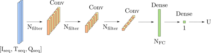
The CNN architecture consisting of 3 convolutional (Conv) layers and one hidden dense layer. By replacing the convolutional layer with a layer of LSTM neurons, the LSTM architecture is designed accordingly
-
Long Short-Term Memory Neural Network (LSTM)
-
Merge Long Short-Term Memory Neural Networks (MergeLSTM)
-
Convolutional Neural Network (CNN)
-
Merge Convolutional Neural Networks (MergeCNN)

Using the “Merge Neural Network” structure, different types of neurons can be investigated, as shown in Fig. 4. By exchanging the upper dense layer with NLSTM neurons, the MergeLSTM is assembled. The LSTM is a promising candidate, as it is designed for processing sequential data, especially for memorizing long-term dependencies (Goodfellow et al. 2017). The output of the LSTM layer is the hidden state, such that in our architecture, the hidden state is merged to the output of the dense layer of the lower branch.
In terms of the MergeCNN, the upper dense layer is replaced by three one-dimensional convolutional layers, to investigate the benefits of using local connectivity and parameter sharing approaches (Goodfellow et al. 2017). By using convolutional filters and corresponding strides, the time dimension of Iseq is compressed in each layer, such that after three layers, the sequence length is reduced to 1. In each layer, the compression and feature extraction is done by Nfilter, such that in the last layer, an output with the depth of Nfilter is produced. This output is flattened and connected to the merge layer. The filter size and convolution stride are set in such a way, that the filter positions do not overlap and no padding or pooling layer needs to be involved. This combination of CNN and sliding window approach is known in the literature as Temporal Convolutional Network (TCN) (Zhou et al. 2020).
As another approach, the sequence of [Iseq,Tseq,Qseq] is used as inputs for an LSTM and CNN. This approach tests the usefulness of the input sequences Tseq and Qseq. For the case of the CNN, the architecture is shown in Fig. 5. In this case, the convolutional layers are still one-dimensional, as the three inputs are organized in the depth dimension. In terms of the LSTM architecture, the convolutional layers are replaced by one hidden LSTM layer.
Evaluation
The evaluation metrics introduced are a measure for comparing the strengths and weaknesses of each individual method. In this work, we concentrate on the performance and model complexity. In addition, from the perspective of a vehicle manufacturer, a special focus is set on a possible application with respect to automotive framework conditions. Automotive frameworks are often restricted to reduced computational capacities and aim at efficient data processing, which needs to be considered for battery modeling of large EV fleets.
Performance
For evaluating the accuracy of the ML models, the root mean squared error (RMSE) in Eq. 2 and mean absolute error (MAE) in Eq. 3 is used.
The parameter N denotes the total number of samples in the validation/testing set, \(\hat {y}_{n}\) is the prediction, and yn the ground-truth. For statistical reasons and to mitigate the effects of randomness, all experiments are repeated an additional time on another randomly drawn data set. The overall performance score of an ML model is then obtained by averaging over the repetitions of all different battery aging states.
Model complexity
The model complexity is divided into processing time and required memory. The processing time is measured during training, validation, and testing of each model, by using the python library time.process_time(). Memory consumption is considered in two process steps. First, the maximum memory peak required to parameterize the ML models during the training phase is determined. Here, the additional memory allocation in the fit call is measured, such that the measurements do not include the size of the data set. The used python library is tracemalloc. Second, the memory required to store the final ML model, which remains on the hard disk, is considered. This memory is needed to run the algorithms on an automotive ECU and is determined by the number of model parameters based on theoretical considerations.
All experiments are carried out on a desktop computer with an Intel I5-8600K CPU with 32 GB RAM. Although neural networks tend to benefit from GPU processing, their impact is negligible using small network architectures and low batch sizes (Goodfellow et al. 2017). Hence, for reasons of comparability, all experiments are performed on a single CPU core.
Hyperparameter tuning
In the first stage of the experiments, hyperparameter tuning is performed individually for each ML method by using the validation set. The main metric for this decision is the RMSE. In all models, the evaluated hyperparameter space is chosen in such a way, that the RMSE shows stagnation effects at some point in the hyperparameter space. Then, only negligible performance gains can be achieved for the more complex models at the expense of higher training and testing times. Therefore, the chosen optimal model is selected in such a way, that it combines near minimal RMSE values with a low as possible model complexity. This approach is also useful to prevent the models from overfitting. Table 1 shows the selection of the optimal hyperparameters with respect to the validation set performance.
As a next stage of the experiments, the optimal models of each ML method are compared by using the testing set.
Results and discussion
The RMSE on the testing set of each optimized ML model is shown graphically in Fig. 6. In combination with the evaluation metrics in Table 2 and the observed training time in Fig. 7, three conclusions can be drawn:
-
1
The neural network models show a significantly better performance than all other regression methods.
Fig. 6 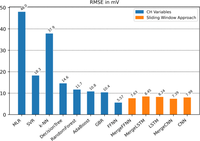
RMSE of the different ML methods using CH variables (blue) or sliding window approach (orange)
Fig. 7 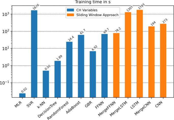
Logarithmic plot of the training time of the ML models in seconds. Although the methods using CH variables (blue) and the sliding window approach (orange) need to process the same amount of data, the training time differs in order of decades
Table 2 Comparison of the performance of the different ML methods -
2
All neural network models using the sliding window approach show a similar performance with respect to the RMSE and MAE.
-
3
The FFNN, which uses the low pass filter variables, shows the best prediction accuracy.


In the following, the characteristics of each ML method are discussed in more detail.
Classical ML methods
As expected, the MLR shows the highest inaccuracies due to the high non-linearities, especially in areas of low SOCs, where a further discharge causes a strong voltage drop in the battery cell. Also, high current excitations are leading to strong mispredictions. Advantages are the low training and testing times and the low model complexity after fitting is complete.
The unsatisfying result of the SVR is due to one main reason: It does not scale well to large data sets, as the computation requirements increase rapidly in the number of training samples (Pedregosa et al. 2011). Therefore, we decide to reduce the training set size of the SVR to one-tenth of the original size. Even for this limited set, the training time is already much higher than for all other methods, excluding LSTMs. Additionally, the training time also heavily depends on the choice of C and ε. Low C and high ε showed training times which are magnitudes lower, but also weaker RMSE scores. Additionally, the SVR shows by far the highest testing times of all models, as the kernel needs to be computed between the new observations and all estimated support vectors (Smola and Schölkopf 2004). Due to this high requirement on computation power, SVR for battery state estimation can not be recommended.
K-NN can also not be recommended, as it shows a low-performance score, together with high testing times. Those high testing times are due to the fact that the distances from a new observation to each training vector need to be calculated. This results in high computational demands, even if the K-D tree structure (Pedregosa et al. 2011) for organizing the training samples is used. Furthermore, the K-NN algorithm requires the entire data set to be permanently stored in memory. Additionally, K-NN does not work well with CH variables, as the PT-1 terms correlate to the current. As a result, the distance calculations are biased towards the current. This problem also occurs in a weakened form with SVR, as the RBF kernel also requires the calculation of a euclidean distance.
The decision tree shows rather unsatisfying RMSE and MAE scores, but very small training and testing times. Even in ensemble methods with roughly 100 trees, the training time stays within a reasonable amount of time. However, decision trees have another drawback: as they produce only piece-wise constant predictions (Pedregosa et al. 2011), they are not well suited for predicting continuous variables like the voltage.
This problem can be greatly mitigated if ensemble methods are used. Of the ensemble methods, both bagging (Random Forest) and boosting approaches (AdaBoost, GBR) show a significant gain in RMSE, from which the gradient boosting approach achieved the largest improvement with approximately 4mV. When comparing the MAE, the ensemble methods even achieve performance close to the neural network models. However, the ensemble methods show a strong increase in memory occupation with approximately 30 MB due to their high amount of parameters. As a consequence, these methods can only be partly recommended for situations where memory is not a critical factor.
Neural network models
Neural networks show better RMSE values than the conventional regression methods and are therefore recommended as the method of choice for battery state estimation. Furthermore, the memory requirements of neural networks are rather small. Based on Table 2, all networks comprise of a low number of parameters, which allows them to be used even in situations where memory is limited. Additionally, due to the training with stochastic gradient descent (SGD), neural networks enable continuous learning, assuming that the network is already trained and new samples are recorded afterwards. To update the neural network, the SGD organizes the new unseen situations into batches and applies them to the next update step. In contrast, all other methods have to start the training from scratch as they require all seen situations for parameter optimization. Hence, the entire data set needs to be allocated in memory.
Regarding the performance, all network architectures, which use the sliding window approach, show similar results. The first observation is that the CNN shows worse results regarding all performance metrics compared to the MergeCNN, whereas the LSTM shows a slightly improved RMSE but a higher computational complexity than the MergeLSTM. Therefore, we can conclude that the inputs Tseq and Qseq are contra-productive, especially regarding the computational requirements. Both variables T(t) and Q(t) are slow-changing, such that for the prediction, the most recent value is sufficient. When not using both variables, the dimensionality of the input is significantly reduced, while keeping all relevant information at the same time.
The LSTMs show the lowest results of the sliding window approaches, which can be attributed to the selected LSTM architecture. The LSTM architecture is kept deliberately simple with a correspondingly slightly lower RMSE in order to maintain the training time within limits. The reason for the high training times in LSTMs is the one-after-another calculation of the hidden state vector, in which the subsequent hidden state requires the previous hidden state to be already computed. Processing a sequence of 100 inputs, therefore, requires 100 updates of the entire LSTM and therefore a massive amount of computations, whereas FFNNs and CNNs can process the sequential input in a single forward pass.
In both MergeFFNN and MergeCNN, additional tests show that the training times are only slightly higher if we increase the sequence length to 200 and beyond. We want to point out that in such a case, more than twice the history of the current can be observed, such that prediction performance can be further improved. This also explains why all sequential networks stagnate at a similar RMSE, as for better performance scores, higher look-backs are required.
The FFNN with CH does not suffer from the problem of a finite look-back, as the PT-1 term is dependent on all past current values, and therefore encompasses information that is out of the range of the sliding window. In our experiments, this enabled the FFNN with CH to achieve the best prediction performance, as shown in Fig. 8. The RMSE of 5.57mV is less than two standard deviations of the sensor noise of the voltage. This performance corresponds to 0.16% with respect to an average battery voltage of 3.6 V. The FFNN also shows smaller training and testing times than the other neural networks. However, as mentioned in “Battery electric modeling” section, the time constants τCH,1 and τCH,2 suffer from the disadvantage of being determined in advance. This can become a problem if the algorithm should be used for a large number of battery cells, as the electric battery behavior changes depending on the construction case, material composition, and aging state.

FFNN performance under automotive driving conditions. The FFNN prediction (orange) achieves an overall RMSE of 5.57 mV compared to the true voltage characteristic (blue)
Therefore, in an additional experiment, the prediction performance of three different FFNN architectures using a non-optimal time constant τCH,2 is investigated. This experiment aims to simulate the case, that the time constant is optimized using a different battery cell. From the results in Fig. 9, we conclude that the area of the optimal time constant is between 100 and 800. Hence, estimating one time constant for multiple battery cells of the same construction can be sufficient.

The performance changes, if the slow history time constant τCH,2 is varied. The test set is used to determine the RMSE for three different FFNN architectures, which are notated as (layer, neurons)
In summary, taking into account the given data set, the performance, and model complexity, the FFNN with the CH is able to provide the greatest potential. However, one should be aware that our data is synthetically generated based on an ECM, which also relies on time constants, as shown in Fig. 2. Therefore, the good result of the FFNN with CH is limited to the precision of the ECM. If the battery cell can be modeled by an ECM with high accuracy, then the FFNN with CH models this ECM with low error, and if both errors are assumed to add up, then the total error would still be small. In such a case, an FFNN with CH can be an extremely effective choice. On the other side, if the ECM itself already shows weaker results in modeling the battery cell, then the assumption is that the time constant-based FFNN will also not perform well. Hence, switching to the sliding window approach can be more beneficial.
The two recommended candidates are MergeFFNN and MergeCNN. From those two possibilities, it should be evaluated whether it is profitable to accept longer training times of the MergeCNN for the gain in performance. In a conclusion, testing all three architectures is recommended, as the performance of the ML algorithm always depends on the individual data situation.
Conclusion
ML models share the ability to learn the electric behavior of automotive battery cells directly from in-vehicle sensor data. As a consequence, expensive laboratory experiments for battery model parametrization is no longer required, which makes data-driven methods interesting for large EV fleets. However, the performance of ML methods highly depends on the application as well as on the given data set. Hence, a comparison among these methods is required beforehand to select the optimal candidate for a given task.
In this work, the advantages and drawbacks of a wide range of possible ML methods for data-driven battery-electric modeling are investigated. In a comprehensive study, each ML method is trained and optimized on a large and qualitative data set, which includes multiple automotive driving profiles, battery SOHs, and a broad temperature range.
By comparing the optimized ML models, all conventional regression methods could not be fully recommended, as each method shows one or multiple disadvantages. As a result, neural networks are found to be superior in terms of model complexity and accuracy, which is consistent with the evaluation of ML methods used in other applications (Chandran et al. 2021). In particular, FFNNs provide the smallest average error deviations of 0.16%, which corresponds to an RMSE of 5.57mV and falls within two standard deviations of the voltage sensor noise. Furthermore, the MergeFFNN and MergeCNN show similar performance using the generalized sliding window approach. Adding the fact of continuous learning renders the neural networks the method of choice for battery state modeling. This key capability keeps the battery models updated with a low computational effort and accounts for changing electrical behavior as the battery ages during operation. Altogether, this high accuracy and continuous learning capability is making neural networks an interesting alternative for future battery electrical modeling approaches.
Future work will test the three architectures on further automotive data sets, which are obtained from real battery cells. In addition, the behavior of the serial combination of multiple cells needs to be evaluated as the next step towards EV battery system modeling.
Availability of data and materials
Due to confidentiality agreements, the utilized battery data cannot be made publicly available.
References
Andersson, M, Johansson M, Klass VL (2020) A continuous-time LPV model for battery state-of-health estimation using real vehicle data In: 2020 IEEE Conference on Control Technology and Applications (CCTA), 692–698.
Breiman, L, Friedman JH, Stone CJ, Olshen RA (1984) Classification and Regression Trees. Chapman and Hall/CRC, Boca Raton, Florida.
Chandran, V, K Patil C, Karthick A, Ganeshaperumal D, Rahim R, Ghosh A (2021) State of charge estimation of lithium-ion battery for electric vehicles using machine learning algorithms. World Electr Veh J 12(1):38.
Choi, W, Shin H-C, Kim JM, Choi J-Y, Yoon W-S (2020) Modeling and applications of electrochemical impedance spectroscopy (EIS) for lithium-ion batteries. J Electrochem Sci Technol 11(1):1–13.
Chollet, F, et al. (2015) Keras. https://keras.io.
Drucker, H (1997) Improving regressors using boosting techniques In: Proceedings of the Fourteenth International Conference on Machine Learning, ICML ’97, 107–115.. Morgan Kaufmann Publishers Inc., San Francisco, CA, USA.
Friedman, JH (2000) Greedy function approximation: A gradient boosting machine. Ann Stat 29:1189–1232.
Goodfellow, I, Bengio Y, Courville A (2017) Deep Learning. MIT Press, Cambridge, MA, USA. http://www.deeplearningbook.org.
Hastie, T, Tibshirani R, Friedman J (2009) The Elements of Statistical Learning - Data Mining, Inference, and Prediction. Springer, Berlin, Heidelberg.
Heinrich, F, Lehmann T, Jonas K, Pruckner M (2021) Data driven approach for battery state estimation based on neural networks In: 14th Conference on Diagnostics in Mechatronic Vehicle Systems, 197–212.
Heinrich, F, Noering FK-D, Pruckner M, Jonas K (2021) Unsupervised data-preprocessing for long short-term memory based battery model under electric vehicle operation. J Energy Storage 38:102598.
Heinrich, F, Pruckner M (2020) Data-driven approach for battery capacity estimation based on in-vehicle driving data and incremental capacity analysis In: Proceedings of 12th International Conference on Applied Energy, Part 2, Thailand/Virtual. Volume 10.
Hu, X, Li S, Peng H (2012) A comparative study of equivalent circuit models for Li-ion batteries. J Power Sources 198:359–367.
International Energy Agency (IEA) (2021) Global EV Outlook 2021. https://www.iea.org/reports/global-ev-outlook-2021. Accessed 30 June 2021.
Ke, G, Meng Q, Finley T, Wang T, Chen W, Ma W, Ye Q, Liu T-Y (2017) LightGBM: A Highly Efficient Gradient Boosting Decision Tree In: Advances in Neural Information Processing Systems, 3146–3154.
Kingma, DP, Ba J (2017) Adam: A Method for Stochastic Optimization. http://arxiv.org/abs/1412.6980.
Klass, V (2015) Battery health estimation in electric vehicles, 59.. KTH Royal Institute of Technology, Stockholm, Applied Electrochemistry.
Li, W, Cao D, Jöst D, Ringbeck F, Kuipers M, Frie F, Sauer DU (2020) Parameter sensitivity analysis of electrochemical model-based battery management systems for lithium-ion batteries. Appl Energy 269:115104.
Li, S, Li J, He H, Wang H (2019) Lithium-ion battery modeling based on big data. Energy Procedia 159:168–173.
Li, P, Zhang Z, Xiong Q, Ding B, Hou J, Luo D, Rong Y, Li S (2020) State-of-health estimation and remaining useful life prediction for the lithium-ion battery based on a variant long short term memory neural network. J Power Sources 459:228069.
Lucu, M, Martinez-Laserna E, Gandiaga I, Camblong H (2018) A critical review on self-adaptive li-ion battery ageing models. J Power Sources 401:85–101.
Orliński, P, Gis M, Bednarski M, Novak N, Samoilenko D, Prokhorenko A (2019) The legitimacy of using hybrid vehicles in urban conditions in relation to empirical studies in the WLTC cycle. J Mach Constr Maint-Problemy Eksploatacji.
Pedregosa, F, Varoquaux G, Gramfort A, Michel V, Thirion B, Grisel O, Blondel M, Prettenhofer P, Weiss R, Dubourg V, Vanderplas J, Passos A, Cournapeau D, Brucher M, Perrot M, Duchesnay E (2011) Scikit-learn: Machine learning in Python. J Mach Learn Res 12:2825–2830.
Severson, KA, Attia PM, Jin N, Perkins N, Jiang B, Yang Z, Chen MH, Aykol M, Herring PK, Fraggedakis D, Bazant MZ, Harris SJ, Chueh WC, Braatz RD (2019) Data-driven prediction of battery cycle life before capacity degradation. Nat Energy 4(5):383–391.
Shen, S, Sadoughi M, Li M, Wang Z, Hu C (2020) Deep convolutional neural networks with ensemble learning and transfer learning for capacity estimation of lithium-ion batteries. Appl Energy 260:114296.
Smola, AJ, Schölkopf B (2004) A tutorial on support vector regression. Stat Comput 14(3):199–222.
Stroe, D, Schaltz E (2020) Lithium-ion battery state-of-health estimation using the incremental capacity analysis technique. IEEE Trans Ind Appl 56(1):678–685.
Tian, H, Qin P, Li K, Zhao Z (2020) A review of the state of health for lithium-ion batteries: Research status and suggestions. J Clean Prod 261:120813.
Vidal, C, Malysz P, Kollmeyer P, Emadi A (2020) Machine learning applied to electrified vehicle battery state of charge and state of health estimation: State-of-the-art. IEEE Access 8:52796–52814.
Volkswagen AG (2021) Volkswagen Power Day 2021. https://www.volkswagenag.com/en/events/2021/Volkswagen_Power_Day.html. Accessed 30 June 2021.
Waldmann, T, Wilka M, Kasper M, Fleischhammer M, Wohlfahrt-Mehrens M (2014) Temperature dependent ageing mechanisms in lithium-ion batteries–a post-mortem study. J Power Sources 262:129–135.
Wang, Y, Tian J, Sun Z, Wang L, Xu R, Li M, Chen Z (2020) A comprehensive review of battery modeling and state estimation approaches for advanced battery management systems. Renew Sust Energ Rev 131:110015.
Wu, B, Widanage WD, Yang S, Liu X (2020) Battery digital twins: Perspectives on the fusion of models, data and artificial intelligence for smart battery management systems. Energy AI 1:100016.
Xiong, R, Li L, Tian J (2018) Towards a smarter battery management system: A critical review on battery state of health monitoring methods. J Power Sources 405:18–29.
You, G, Park S, Oh D (2016) Real-time state-of-health estimation for electric vehicle batteries: A data-driven approach. Appl Energy 176:92–103.
Zhang, Y, Harb JN (2013) Performance characteristics of lithium coin cells for use in wireless sensing systems: Transient behavior during pulse discharge. J Power Sources 229:299–307.
Zhang, J, Lee J (2011) A review on prognostics and health monitoring of li-ion battery. J Power Sources 196(15):6007–6014.
Zhang, X, Lu J, Yuan S, Yang J, Zhou X (2017) A novel method for identification of lithium-ion battery equivalent circuit model parameters considering electrochemical properties. J Power Sources 345:21–29.
Zhou, D, Li Z, Zhu J, Zhang H, Hou L (2020) State of health monitoring and remaining useful life prediction of lithium-ion batteries based on temporal convolutional network. IEEE Access 8:53307–53320.
About this supplement
This article has been published as part of Energy Informatics Volume 4 Supplement 3, 2021: Proceedings of the 10th DACH+ Conference on Energy Informatics. The full contents of the supplement are available online at https://energyinformatics.springeropen.com/articles/supplements/volume-4-supplement-3.
Funding
Publication funding was provided by the German Federal Ministry for Economic Affairs and Energy.
Author information
Authors and Affiliations
Contributions
FH: Conceptualization, Methodology, Data Acquisition, Analysis, Writing - original draft. PK: Software, Analysis, Writing - original draft. MP: Conceptualization, Supervision, Writing - review, and editing. All authors read and approved the final manuscript.
Corresponding author
Ethics declarations
Competing interests
The authors declare that they have no known competing financial interests or personal relationships that could have appeared to influence the work reported in this paper.
Additional information
Publisher’s Note
Springer Nature remains neutral with regard to jurisdictional claims in published maps and institutional affiliations.
Rights and permissions
Open Access This article is licensed under a Creative Commons Attribution 4.0 International License, which permits use, sharing, adaptation, distribution and reproduction in any medium or format, as long as you give appropriate credit to the original author(s) and the source, provide a link to the Creative Commons licence, and indicate if changes were made. The images or other third party material in this article are included in the article’s Creative Commons licence, unless indicated otherwise in a credit line to the material. If material is not included in the article’s Creative Commons licence and your intended use is not permitted by statutory regulation or exceeds the permitted use, you will need to obtain permission directly from the copyright holder. To view a copy of this licence, visit http://creativecommons.org/licenses/by/4.0/.
About this article

Cite this article
Heinrich, F., Klapper, P. & Pruckner, M. A comprehensive study on battery electric modeling approaches based on machine learning. Energy Inform 4 (Suppl 3), 17 (2021). https://doi.org/10.1186/s42162-021-00171-7
Published:
DOI: https://doi.org/10.1186/s42162-021-00171-7