Towards domain-specific surrogate models for smart grid co-simulation

Abstract

Surrogate models are used to reduce the computational effort required to simulate complex systems. The power grid can be considered as such a complex system with a large number of interdependent inputs. With artificial neural networks and deep learning, it is possible to build high-dimensional approximation models. However, a large data set is also required for the training process. This paper presents an approach to sample input data and create a deep learning surrogate model for a low voltage grid. Challenges are discussed and the model is evaluated under different conditions. The results show that the model performs well from a machine learning point of view, but has domain-specific weaknesses.

Introduction

As a safety-critical infrastructure, the power grid is not suitable for testing new algorithms or other technologies. At the same time, there is no test system that is comparable to the power grid in terms of functionality and behavior (Nieße et al. 2014). Simulation and co-simulation are therefore key tools for the development and testing of new technologies and methods to transform the power grid into a smart grid. In general, a distinction is made between static and dynamic power grid simulation. In the static simulation, a steady state analysis is performed. In a dynamic simulation, however, transient effects can be observed. An important factor for simulation systems is the time required for the simulation. Frequent questions include: Does the simulation end in reasonable time? Is a step computable in real time (or even faster)? In small systems (e.g. a small distribution grid), runtime may not be a real issue. In larger simulation systems (e.g. the entire German transmission grid), however, time becomes a critical factor.

A possible solution to the problem are surrogate models, i.e. data-driven approximations of the system to be simulated. The use of a surrogate model represents a trade-off between accuracy and runtime of the system. Many components can be involved in power grid simulation systems, such as photovoltaic (PV) panels, combined heat and power (CHP) plants, consumers such as households or commercial facilities. In steady state simulation, some components can be replaced by time series because their behavior is not controllable. However, others can reduce or increase consumption or generation to ensure a stable state of the grid.

In order to simulate a typical low voltage (LV) grid, household models, PV or CHP models at household level, and models of smaller commercial facilities may be needed (Papathanassiou et al. 2005). The simulation of such a LV grid can take a while, even if some components are replaced by time series. The total runtime depends on the time resolution and the number of simulation steps. For instance, the simulation system used in this paper took about 15 min to simulate a year with time steps of 15 min. The next step for a large-scale simulation is to connect several of those LV grids to a medium voltage (MV) grid. Then PV or wind farms and larger commercial or industrial facilities are added (Buchholz et al. 2004). The resulting simulation system may not be simulated in reasonable time. Replacing individual components with surrogate models is a less promising approach. The components themselves are not that slow and the time-consuming part is the need to simulate a large number of components (Koch et al.).

This paper proposes to replace whole LV grids with a single surrogate model built with a deep neural network. This includes the components connected to the grid. As described in Balduin (2018), the idea is to integrate domain knowledge and characteristics of the power grid into the surrogate modeling process. The grid has a large number of inputs with strong interactions, such as load and generation, which may depend on consumer behavior or weather conditions. Information about the simulation setup and interdependencies of the components should be used to reduce the dimensionality of the problem. The individual components are to be abstracted by a correlation model built from this information. The contribution of this paper is to provide a benchmark model and evaluation environment. This model is built without domain knowledge. The suitability of the model is investigated in various simulation experiments, which represent the evaluation environment.

The rest of this paper is structured as follows: “Related work” section provides a brief introduction to surrogate models, deep learning, power grid simulation, and power flow calculations. In addition, related work in the field of surrogate models for the power grid will be presented. “Methodology” section presents the simulation setup and describes the construction of the deep learning model. Furthermore, the experimental setup and hypothesis are defined. In “Building the model” section, sampling and model building is documented. “Case study” section documents the conduct of the case study and “Conclusion and outlook” section concludes this paper and presents future work.

Related work

Surrogate modeling is well documented in the literature, e.g. in Myers et al. (2016); Kleijnen (2015), or Siebertz et al. (2017). An approximation function y=f(x₁,x₂,…,x_k)+ε is called a surrogate model. The x_i are the inputs, y marks an output, and ε is the error between f and the true but unknown response function. A sample is an arbitrary, but fixed assignment of the inputs and the corresponding output of the real system. f is built with a sufficient number of samples, called the training data set. One way to create a surrogate model is machine learning, e.g. nearest neighbors, support vector machines, or artificial neural networks (ANN). But there are also other methods and each has advantages and disadvantages. In the German research project D-Flex (Koch et al.) a large simulation with ten thousands of simulation models were carried out to compare different approaches for the integration of renewable energy resources. After some benchmarks, parts of the simulation models were replaced by look-up tables. Only by using these surrogate models was it possible to complete the simulations in a reasonable time. Nevertheless, thousands of simulation models were replaced by the same number of surrogate models. Although this was sufficient for the project, it is not an optimal approach.

Artificial neural networks

With the increasing computational power, ANNs and deep learning can be used to achieve impressing results on various tasks in different fields¹. An ANN is able to approximate any continuous function (Csáji 2001). The basic idea of an ANN is shown in Fig. 1.

Fig. 1

Fully connected ANN with three input neurons, two output neurons, and one hidden layer (l.). Activation functions (r.) from top to bottom: identity, sigmoid and ReLU. In each of the neurons, a weighted sum is calculated and sent through an activation function as output to the next layer of neurons. The activation function defines how the output is forwarded (Schmidhuber 2015). Backpropagation is used to adjust the weights of the network to the current output error (Rumelhart et al. 1988)

ANNs have a long history and by now there are many different types. In a feed forward network (Schmidhuber 2015), all connections between neurons are only in forward direction towards the output layer. A recurrent neural network (Elman 1990) also allows connections back towards the input layer. This enables the network to memorize earlier inputs and not just the current input. More recent types of ANNs are the convolutional neural network (Fukushima 1980), which is often used for image classification and long short-term memory networks (Hochreiter and Schmidhuber 1997), which are good for time series predictions. These types are often associated with the term deep learning, which means that the neural network has many hidden layers (Schmidhuber 2015, p. 7). Some tools for deep learning are listed in Bridgewater ().

Power system simulation

The simulation of the electrical power system is used for different applications like long-term generation and transmission expansion planning, short-term operational simulations, or market analysis. In many cases it is sufficient to assume that the power grid is in a steady state (Biswas and Das 2011), i.e. transient behavior which results in frequency changes and similar effects are neglected. These effects are either too small or happen too fast to consider them during operation planning of the power grid. The constant-frequency assumption only holds as long as these effects are under control and therefore the dynamic analysis of the power grid is important, too (Elrazaz and Sinha 1979). However, this work focuses on the steady state operation of the power grid.

The main part of steady state analysis is the power flow (PF) analysis. PF is used to calculate bus voltages, currents, active and reactive power flows on the lines as well as line and transformer losses. The most common methods to solve PF problems are the Newton-Raphson (NR) and Gauss-Seidel (GS) methods (Baghaee et al. 2018). Both require an initial guessing of unknown values, which will be iteratively adapted, until the method converges due to some condition. However, bad guessing can lead to the methods not converging and then the calculation has to be repeated.

There are various tools for power system simulation on different abstraction levels. The commercial simulation software PowerFactory of the German company DIgSILENT provides a broad range of functionality and simulation models, from load flow calculations used in steady state analysis to frequency analysis and quasi-dynamic simulation. Similar to PowerFactory is NEPLAN of the Swiss company NEPLAN AG, which also has models integrated and enables static as well as dynamic analysis of the power grid. MATPOWER is an open source toolbox for MATLAB and Octave for steady state power system simulation and optimization. The open-source tool pandapower (Thurner et al. 2018), a joint development of the University of Kassel and Fraunhofer Institute for Energy Economics and Energy System Technology, provides steady state power system modeling, analysis and optimization with load flow calculations and several predefined benchmark grids.

Simulation approaches

The simulation of a system like the smart grid raises new requirements, since multiple domains have to be considered. Besides the more traditional power grid simulation approaches in the previous section, the simulation of the communication system also has to be considered and there are different approaches to face these challenges. A short overview of these approaches follows. However, a more detailed discussion is given by Steinbrink et al. (2017). The idea of multi-domain simulation is to adapt all required simulators to the system of the multi-domain simulation framework. This is advantageous for performance assessment, but Steinbrink et al. argue that much effort is required to adapt or even reformulate the simulator to the target simulation framework. Tools for multi-domain simulation are the Ptolemy II framework or the Modelica language. Another approach is the coordinated simulation (co-simulation), where each simulator is executed in its own runtime environment. The task of a co-simulation framework is to orchestrate these simulators and enable data exchange between them. The separation of modeling and simulation is the major benefit of co-simulation according to Steinbrink et al., since simulation models can be developed by domain experts in environments of their choice and easily reused by others utilizing co-simulation. Examples for co-simulation tools are (again) Ptolemy II and mosaik², developed at OFFIS in Germany. The third approach is real-time simulation, which is commonly used when hardware is involved (hardware-in-the-loop). This allows to test and validate single hardware components without deploying them in the field.

Applications of surrogate models in the energy domain

Various applications of surrogate models in the energy domain can be found. Some of them do not use machine learning. Patsalides et al. presented a simplified distribution grid model (SDGM) to investigate voltage variation and PV capacity in a distribution grid (Patsalides et al. 2015). The SDGM makes use of Thevenin equivalent circuits (TEC), which consist of a voltage source and impedance according to Thevenin’s theorem (Brittain 1990). The authors used the TEC to replace a medium voltage grid. Several regulation algorithms were applied to their model to evaluate penetration of distributed generation. Cha et al. replaced parts of the Bornholm power system (Cha et al. 2012). The authors used the frequency dependent network equivalent method to build a generic model for real time dynamic simulation. Their model achieves high accuracy in several simulations. Model order reduction (MOR) is done to reduce the dimensionality of distribution grid simulations. Li et al. developed a state-space model of a distribution grid for the MOR application (Li et al. 2013). The model was evaluated in several simulations using a the CIGRE benchmark low voltage grid. The authors showed, that their model can compete with other similar approaches, namely the modified nodal analysis.

Other authors used machine learning to build surrogate models. Fikri et al. (2018) compare traditional (i.e. numerical) methods to solve PF calculations with an artificial intelligence method using ANNs. The authors used one ANN each for voltage magnitudes and voltage angles. They conclude that errors between numerical methods and the ANNs are very small on the IEEE 14 bus system, which was used as benchmark. A more comprehensive study is done by Baghaee et al. (2018), who compared even more PF methods with a radial basis function ANN. The authors aim to not only provide a comparison regarding accuracy and performance, but also regarding authenticity and robustness. Both works present promising results and especially for large-scale simulation it is important to reduce the time for PF calculations and increase their robustness. However, the load-flow calculation may not be the only critical factor in large-scale simulations.

The classification of feasible schedules for the flexibility provision in a virtual power plant can be done for single components individually. But Fröhling (2017) proposed a method to solve this problem for coalitions of components utilizing correlations between the components. The idea of forming coalitions of components can be found in other works, too. Blank (2015) used coalitions of renewable power units to access their reliability for the provision of ancillary services. Using the notion of coalitions is a promising approach for combining several models together with a power grid simulation. The first steps towards this approach is presented in the following chapters.

Methodology

The research in this paper is done in the context of the steady state analysis of a power grid (see Fig. 2) and is part of a PhD project (Balduin 2018). Therefore, the approaches presented are quite basic and serve as experimental platform and proof-of-concept for future work. The leading questions for this part of the research are:

• 1 How much runtime performance gain can be expected when a surrogate model replaces a low voltage grid?

  Fig. 2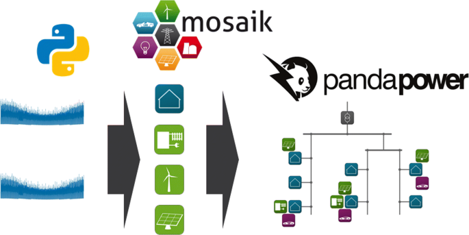

  

  The general setup for the research in this work. Different components are involved, not all of which have been considered in this paper. However, these are still important for future work

• 2 How accurate is a surrogate model that replaces a low voltage grid?

The work done aims to answer these questions and serve as a reference for future work. This section describes the experiments, starting with the simulation setup. This is followed by a description of the neural network architecture. The section concludes with experimental design and hypothesis.

The simulation setup

The first step is the selection of a power grid model and simulator. The python package pandapower is a static power grid simulator and provides several pre-configured grids with different voltage levels. One of those grids is the CIGRE low voltage benchmark grid (Papathanassiou et al. 2005), shown in Fig. 3.

Fig. 3

The CIGRE LV benchmark grid, inspired by: https://github.com/lthurner/ pandapower/blob/v1.3.0/doc/pics/cigre_network_lv.png

The grid consists of 3 areas: a residential subgrid, an industrial subgrid, and a commercial subgrid. This work will mainly focus on the residential subgrid. Nonetheless, the other areas are also modeled and may be considered in future work. In the residential subgrid, the grid has 5 loads (at bus bars R11, R15, R16, R17, R18), which are either residential consumers or apartment buildings. These households are modeled by different time series taken from the German research project Smart Nord³. In the current version, the models take a value from the time series assigned to them at each step and forward it. The industrial and commercial grids function in the same way, but are initially only supplied with data from reference years for different commercial buildings. The data and can be downloaded for free on openei.org⁴. The overall load and the proportions of residential and commercial loads are shown in Fig. 4.

Fig. 4

The total load is shown in the top. In the bottom left, the aggregated residential load is shown and in the bottom right, the aggregated commercial load is shown. All data have a 15-min resolution

Since every household has its own time series, no matter if it is residential or part of the apartment, these loads need to be aggregated somehow. Therefore, an aggregation model is integrated in the simulation setup. This model adds up all loads connected to it and forwards the aggregated values to their associated bus bar of the power grid model. Additionally, for each consumer a reactive power value Q is calculated with Q=P· tanφ, assuming a constant cosφ=0.9 for simplification (Schulz et al. 2010).

All models are plugged together using the co-simulation framework mosaik. The co-simulation approach enables to cheaply extend the setup by other simulators as well as to use the surrogate model instead of the grid and other models. The whole setup is shown in Fig. 5.

Fig. 5

The simulation setup. The time series are connected to simple household models, which are connected via aggregator models to the power grid. All the communication is handled by mosaik. Everything in the dashed box is to be replaced by a surrogate model

On the output side, every information that pandapower provides regarding the trafos, buses, lines and loads is collected. Since not all of this information is required for the experiments, only the relevant outputs bus voltage magnitudes per unit (vm_pu) are selected for the surrogate model.

The deep neural network architecture

There are many possibilities to configure a neural network like number of layers and neurons per layer as well as modifications for the training process like training epochs or batch size. Additionally, there are different types of layers and activation functions. For this work, a rather simple architecture is chosen.

Only dense (i. e. fully connected) layers and the rectified linear unit (ReLU) as activation function are used, since the main goal is a proof-of-concept. The number of hidden layers and training epochs will be optimized using a random search cross validation approach. The definition of the number of neurons per layer is not directly part of the cross validation. They are rather calculated depending on the number of layers. There is no general rule for the number of neurons per layer, only rules-of-thumb and recommendations. Heaton (2008) recommended to start with a number of hidden neurons somewhere between the number of input neurons and the number of output neurons. Following this recommendation, the number of neurons n_k of hidden layer k is calculated depending on the number of input neurons n_in, the number of output neurons n_out, and the number of hidden layers hl using the following formula assuming at least one hidden layer:

$$\begin{array}{@{}rcl@{}} n_{k} = \lfloor n_{in} + \frac{n_{out} - n_{in}}{hl+1} \cdot k \rfloor, \textrm{ with}\ hl > 0 \end{array} $$

(1)

In Fig. 6 an example architecture is shown. For higher number of hidden layers, formula 1 results in more hidden neurons than recommended. Nonetheless, cross validation will find a suitable architecture.

Fig. 6

Example ANN architecture with input size n_in=8, output size n_out=2 and two hidden layers. The hidden layer sizes are calculated using formular 1

Experimental setup

A simulation study with domain-independent as well as domain-specific experiments is conducted to answer the research questions from the beginning of this section. The following subsections describe how the experiments are conducted.

Domain-independent experiments

The first experiments cover the general capabilities of the surrogate model as regressor for the simulation model under study. The first criteria of interest is the performance gain. Therefore, the time required for the simulation is measured for both the simulation model and the surrogate model. As shown in Fig. 5, the surrogate model also substitutes some of the connections that require data exchange in the original setup. Since the focus is on the total time of the simulation, this is used as an additional advantage.

The second criteria is the accuracy of the model. The accuracy will be measured with the normalized root mean squared error (NRMSE) between the real y and the predicted output $\tilde {y}$ over all outputs n. First, the RMSE is calculated according Eq. 2 and then normalized with the range of the real output (see Eq. 3).

$$\begin{array}{@{}rcl@{}} \textrm{RMSE }(\tilde{y}, ~ y) &=& \sqrt{\frac{1}{n} \cdot \sum_{i}^{n} (\tilde{y} - y)^{2}} \end{array} $$

(2)

$$\begin{array}{@{}rcl@{}} \textrm{NRMSE }(\tilde{y}, ~ y) &=& \frac{\textrm{RMSE }(\tilde{y}, ~ y)}{y_{max} - y_{min}} \end{array} $$

(3)

The normalization allows the error to be expressed as a percentage value. According to Forrester (2008), a good surrogate model has an NRMSE <10%, which will be used as benchmark.

Summarized, the objectives of the first experiment are a) to gain insight into possible speed-up factors in this (simple) setting, b) to determine the influence of the duration of the simulation – in this case the number of simulated days – on the speed-up and c) to measure the regression capabilities of the surrogate model according to the NRMSE. For the first two objectives, following hypotheses will be tested against a significance level of α=5%:

Hypothesis 1 (Simulation time comparison):

The average time $\bar {t}_{surrogate}$ the surrogate model needs to simulate is significantly shorter than the normal runtime $\bar {t}_{sim}$ (without the surrogate model).

• H₀: $\bar {t}_{surrogate} \geq \bar {t}_{sim}$

• H₁: $\bar {t}_{surrogate} < \bar {t}_{sim}$

Hypothesis 2 (Speed-up comparison):

The speed-up s_i for i simulated days is significantly different from the speed-up s_j for j simulated days.

• H₀: s_i=s_j with i≠j

• H₁: s_i≠s_j with i≠j

Both, the simulation model and the surrogate model, are run for different numbers of simulated days repeatedly. The speed-up for each number of simulated days is calculated. The third objective will be discussed on the basis of the NRMSE at each bus and overall.

Hypothesis 3 (Normalized RMSE):

The error of the surrogate model a) for each bus NRMSE _i and b) overall NRMSE _all is less than 10%.

• H₀: a) ∃i: NRMSE _i≥0.1 b) NRMSE _all≥0.1

• H₁: a) ∀i: NRMSE _i<0.1 b) NRMSE _all<0.1

The two parts a) and b) of hypothesis 3 will be considered separately later.

Domain-specific experiment

In the second experiment, a domain-specific accuracy analysis is done. From an operational view, the nominal voltage U_N should be maintained depending on the grid level. The European standard EN 50160 allows a deviation of the actual voltage U of ± 10%, from which 4% is intended for the MV grid, 2% for the MV-LV transformer and another 4% for the LV grid. Exceeding these limits can damage electrical devices, which must be avoided in any case. During load forecasting, voltage limit violations must be detected in order to avoid them in the real grid. Assuming that the simulation model is able to detect such critical situations, the surrogate model should be able to detect these situations, too.

The detection of critical situations can be seen as classification problem. A critical situation is regarded as positive outcome, but it could also be the other way round. A common metric for such tasks is the confusion matrix (Visa et al. 2011), seen in Fig. 7. Each prediction of the model can classified as exactly one of 4 outcomes: true positive (TP), true negative (TN), false positive (FP) and false negative (FN).

Fig. 7

Confusion matrix for two classes true and false. The result of each classification task can be classified in one of these 4 categories. The results for each category are summed up for further calculations

The confusion matrix is basis for the following measures: accuracy (Eq. 4), precision (Eq. 5), recall (Eq. 6), and F1-score (Eq. 7).

$$\begin{array}{@{}rcl@{}} \text{Accuracy} &=& \frac{TP + TN}{TP + TN + FP + FN} \end{array} $$

(4)

$$\begin{array}{@{}rcl@{}} \text{Precision} &=& \frac{TP}{TP + FP} \end{array} $$

(5)

$$\begin{array}{@{}rcl@{}} \text{Recall} &=& \frac{TP}{TP + FN} \end{array} $$

(6)

$$\begin{array}{@{}rcl@{}} \textrm{F1-score} &=& 2 \cdot \frac{\text{Precision} \cdot \text{Recall}}{\text{Precision} + \text{Recall}} \end{array} $$

(7)

The accuracy takes into account all 4 classes and is an indicator for the overall classification capabilities. However, the accuracy requires both classes to be balanced in the actual data. The precision measures the quality of the predictions with class true, i.e. which part of true predictions actually were true. The recall measures the quality of the model not to miss any true class. The decision between precision and recall depends on how critical false positives respectively false negatives are. If both are considered equally important, the F1-score can be used, which is the harmonic mean of precision and recall.

From a domain point-of-view, false negatives (not detecting a critical situation) are worse than false positives (classifying a situation as critical which is not critical). Therefore, the objective for the second experiment is to measure the capabilities of the surrogate model to detect critical situations according to the recall measure. Nonetheless, the results of the other measures will be provided, too. As concrete use case the bus R18 of the CIGRE LV grid is investigated as well as the buses on the path to bus R1. In Fig. 8 the annual voltage curve of bus R18 is shown.

Fig. 8

Voltage curve of bus R18 for one year. The dotted lines are the voltage boundaries ±4%

From this figure it can be seen that there are several critical situation at Bus R18. However, compared to the total amount of steps, very few critical situations exist. Both models will be compared not only at bus R18, but also on at the other buses on the path to R1 and the task is, to correctly classify, if a situation is critical. For this first attempt the model should achieve a recall of 75% to be significantly better than random guessing⁵.

Hypothesis 4 (Detection of critical situations):

The surrogate model is able to correctly classify critical situations with a recall of at least 75%.

• H₀: recall <0.75

• H₁: recall ≥0.75

This experiment will not be repeated. All components are deterministic and the outputs only change with different inputs.

Building the model

A surrogate model must be built as a prerequisite for both experiments. The first step in this process is to generate training data. Simulation data that could be used for training is limited. Therefore, it would be better to have a sampling function to generate any number of samples. In general, a good first approach is to identify all relevant inputs of the system and their valid value ranges. Then, input combinations can be drawn using sampling designs such as Monte Carlo or Latin Hypercube. These inputs are fed to the system to generate the corresponding output. In the following, this approach will be referred to as pure random sampling. However, initial attempts using pure random sampling resulted in the PF calculation of pandapower not converging.

There are several reasons why this did not work for the current case. Pure random sampling assumes to have uniformly or even normally distributed input data. Figure 9 shows an example of the simulation data for a consumer (a household). The data of this consumer are neither uniformly nor normally distributed. Data from other households are similarly shaped. Therefore, such distributions do not represent the input data.

Fig. 9

Histogram with 200 bins showing the distribution of one household’s load over one year. Like the other households in the dataset, this household has a low mean value (0.38 kW) and a high maximum value (22.92 kW). Every value above 2 or 3 kW can be considered as peak load event. Using a normal or even uniform distribution increases the likelihood of peak loads in any household. This also increases the probability of peak loads occurring in many households at the same time. The result would be an overload of the grid

Instead of finding a suitable distribution for the inputs a kernel density estimation (KDE) is applied. The python library scipy provides Gaussian KDE which uses Scott’s rule of thumb (Scott 1992, p. 55) to automatically determine the bandwidth. The KDE function is computed for each input individually. Samples are now drawn from the KDE function. This makes it possible to draw any number of samples as training data. Figure 10 shows the KDE and samples from KDE for the household from Fig. 9.

Fig. 10

Gaussian KDE (green line) applied to household data (blue dotted line). Samples for one year drawn from the KDE function (orange dashed line). The area between 0.0 and 0.75 kW is smoothed a bit too much. Overall, however, the estimate seems to fit

Using KDE, 50,000 samples were taken and used as training data. However, the model was not able to detect critical situations at all. As a workaround, 25,000 KDE samples were used and another 25,000 samples from the time series (the last ≈260 days of the year) were added to the training data for the final model. The remaining 100 days were left as test data. Five-fold cross-validation was applied on the training data, i.e. 40,000 samples were used as training data and 10,000 as validation data in each run.

During the training process, 2 hyperparameters were optimized: hidden layers and training epochs. The random search algorithm could chose between 1 and 15 layers and between 6 and 12 epochs. The training took about 10 hours on dedicated hardware including random search and cross-validation. The final architecture of the neural network consists of 14 hidden layers (see Fig. 11) and was trained for 11 epochs.

Fig. 11

Architecture of the neural network after the training process with random-based hyper parameter tuning and cross validation. The model consists of fourteen hidden layers. The 76 inputs are all P-Q pairs for the loads. Outputs are voltage values for 44 buses

Case study

In a case study, the simulation model (Fig. 5) and the surrogate model (described in the previous section) were compared. Three domain-independent experiments were conducted and are presented in the following. All experiments were carried out on a Windows 10 machine with an Intel Core i7-7820HQ 2.90 GHz CPU and 16 GB RAM. The domain-dependent experiment is documented at the end of this section.

Simulation time comparison In the first experiment (hypothesis 1), both models are repeatedly run for 10 simulated days. Table 1 shows the experiment summary and the analysis of variance (ANOVA). The average runtime of the simulation model is $\bar {t}_{sim} = 22.2$ seconds. For the surrogate model, the average runtime is $\bar {t}_{surrogate} = 7.7$ seconds. This results in a speed-up of $\frac {22.2s}{7.7s} = 2.88$. Furthermore, $\bar {t}_{sim}$ and $\bar {t}_{surrogate}$ are apparently different. ANOVA shows that this difference is significant: p=1.82·10⁻³⁶<0.05=α. Therefore, the null hypothesis $\bar {t}_{surrogate} = \bar {t}_{sim}$ can be rejected.

Table 1 Comparison of the simulation time in seconds with and without surrogate model in the upper table

Speed-up comparison In the next experiment (hypothesis 2), both models are run for 1, 5, 10, 50, 100, and 250 simulated days in a row 10 times repeated. This is done similar to the previous experiment. The speed-up is calculated for each element in one group, i. e. with the same number of simulated days. This results in one 100 samples (= speed-up values) per group. Table 2 shows the simulation summary and the ANOVA. The average speed-ups are between 2.54 and 2.76 and the overall average is 2.65 with standard deviation of $\sqrt {0.033825} \approx 0.18$. There is only a weak correlation between speed-up and the number of simulated days (Pearson correlation is 0.28). However, the ANOVA shows that the differences between speed-ups are statistically significant: p=2.85·10⁻²⁴<0.05 and therefore the null hypothesis can be rejected.

Table 2 Summary of the speed-ups is shown in the upper table

Normalized RMSE In the last domain-independent experiment (hypothesis 3), the accuracy of the models was evaluated. The first 3 months of the year (the part of the data not used for training) were uses as test period. The outputs of the simulation model and the surrogate model were compared with the NRMSE for each bus individually and in total. Table 3 shows the results. Of 44 error values, 13 are >10%, 10 of which are in the commercial and industrial subgrids. This is a good result for the residential subgrids, which is the focus of this work. Nevertheless, part a) of the null hypothesis cannot be rejected. The overall error of 7.5% is lower than the presumed 10% for part b) of the hypothesis. Therefore, the null hypothesis b) can be rejected and the model regarded as good. In particular, the error values of the buses R0 to R10 and R18 indicate that the model is good enough for the domain-specific experiment.

Table 3 Normalized RMSEs for all buses

Detection of critical situations

The last experiment (hypothesis 4) examines the surrogate model’s ability to predict critical situations. Simulation model and surrogate model are compared for 8640 simulation steps (3 simulated months or 90 simulated days). Only the buses R0 to R10 and R18 are considered. Whenever the simulation model outputs a value between 0.96 and 1.04 for a time step, the network state is uncritical (negative event). All other values are considered critical (positive event). In particular, the surrogate model must correctly predict these critical values. The confusion matrix and derived measures are shown in Table 4.

Table 4 Summary of the domain-specific experiment

The accuracy of the model achieves very high values (>0.99). However, since bus voltages are not critical in most cases (true negatives), the accuracy metric is a poor indicator of model quality. Precision measures the proportion of critical situations identified from the surrogate model that were actually critical. The total precision is ≈18%, which indicates a high false positive rate. Especially the result of bus R18 is bad, because not a single critical situation was detected there. More important than precision is recall, which quantifies the rate of undiscovered critical situation. The surrogate model has a total recall rating of ≈31%, which is even worse than random guessing. Therefore, the null hypothesis cannot be rejected. For illustration the simulation results of one day with critical situations for the buses R5, R10, and R18 are shown in Fig. 12.

Fig. 12

Simulation results for buses R5, R10, and R18. Visually, the match between simulation model and surrogate model at buses R5 and R10 is quite good. The third graph reveals that the surrogate model has fundamental problems to reproduce the results for bus R18, which could be a reason for the bad recall rating

Conclusion and outlook

In this paper an approach was presented to replace an entire low voltage grid including the connected components. A deep neural network was used as the surrogate model. Challenges in sampling inputs for the grid were discussed. The capabilities of the surrogate model were evaluated domain-independently in experiments to runtime, speed-up, and accuracy according to the (normalized) RMSE. It has been demonstrated that a) the surrogate model is faster than the simulation model with an average speed-up factor of 2.65 and b) the speed-up factor varies when changing the duration of the simulation and c) the forecasts of the surrogate model show an error of 7% when using the NRMSE. In a domain-specific experiment, the model’s ability to detect critical situations in which the bus voltage exceeds certain limits was investigated. The task was formulated as a classification task. The model should have as low a false negatives rate as possible to detect any critical situation. Therefore, the recall metric was applied to the output of both models for certain buses of interest. The recall rating for these buses was 31%, which is worse than random guessing.

The results lead to the following conclusions. The general capabilities of the surrogate model are quite satisfactory for a first approach with only a simple architecture. One task for future work will be how the model performs when changing the size of the power grid and when adding distributed energy resources such as PV and CHP generation. In particular, the impacts on runtime, speed-up and accuracy are of interest. However, the domain-specific capabilities were not sufficient and the reasons for this can be assumed in the sampling procedure. One approach would be to use more “real” load data to capture their behavior, but this is not always feasible. A more promising approach would be to model the grid inputs as distributions like it is done for probabilistic load flow calculations (Chen et al. 2008). Load dependencies have also not yet been taken into account. The derivation of a correlation graph from the interdependencies between these inputs and the provision as additional information for the model is the goal and part of the future work.

References

Baghaee, HR, Mirsalim M, Gharehpetian GB, Talebi HA (2018) Generalized three phase robust load-flow for radial and meshed power systems with and without uncertainty in energy resources using dynamic radial basis functions neural networks. J Clean Prod 174:96–113.
Balduin, S (2018) Surrogate models for composed simulation models in energy systems. Energy Inform 1(1):30.
Biswas, MM, Das KK (2011) Steady state stability analysis of power system under various fault conditions. Glob J Res Eng 11(6-F).
Blank, D-MM (2015) Reliability assessment of coalitions for the provision of ancillary services. PhD thesis, University of Oldenburg.
Bridgewater, AAn overview of deep learning tools. https://www.computerweekly.com/news/252452432/An-overview-of-deep-learning-tools.
Brittain, J (1990) Thevenin’s theorem. IEEE Spectr 27(3):42.
Buchholz, B, Frey H, Lewald N, Stephanblome T, Styczynski Z (2004) Advanced planning and operation of dispersed generation ensuring power quality security and efficiency in distribution systems. CIGRE 2004 Session, Citeseer, Paris.
Cha, ST, Wu Q, Østergaard J (2012) A generic danish distribution grid model for smart grid technology testing In: 2012 3rd IEEE PES Innovative Smart Grid Technologies Europe (ISGT Europe), 1–6.. IEEE, Piscataway.
Chen, P, Chen Z, Bak-Jensen B (2008) Probabilistic load flow: A review In: 2008 Third International Conference on Electric Utility Deregulation and Restructuring and Power Technologies, 1586–1591.. IEEE, Piscataway.
Csáji, BC (2001) Approximation with artificial neural networks, vol. 24. Faculty of Sciences, Etvs Lornd University, Hungary.
Elman, JL (1990) Finding structure in time. Cogn Sci 14(2):179–211.
Koch, M, Ritter D, Bauknecht D, et al.Dezentral und zentral gesteuertes Energiemanagement auf Verteilnetzebene zur Systemintegration erneuerbarer Energien–Wissenschaftlicher Endbericht. https://www.offis.de/offis/projekt/d-flex.html.
Elrazaz, Z, Sinha N (1979) Modelling and simulation of power system for dynamic analysis. IFAC Proc Vol 12(5):204–211.
Fikri, M, Haidi T, Cheddadi B, Sabri O, Majdoub M, Belfqih A (2018) Power flow calculations by deterministic methods and artificial intelligence method. Int J Adv Eng Res Sci 5:148–152.
Fröhling, J (2017) Abstract flexibility description for virtual power plant scheduling. PhD thesis, BIS der Universität Oldenburg.
Fukushima, K (1980) Neocognitron: A self-organizing neural network model for a mechanism of pattern recognition unaffected by shift in position. Biol Cybern 36(4):193–202.
Forrester, A, Sobester A, Keane A (2008) Engineering design via surrogate modelling: a practical guide, 1st edn. Wiley, Chichester, West Sussex.
Heaton, J (2008) Introduction to neural networks with java, 2nd edn. Heaton Research, Inc, Chesterfield.
Hochreiter, S, Schmidhuber J (1997) Long short-term memory. Neural Comput 9(8):1735–1780.
Kleijnen, JPC (2015) Design and analysis of simulation experiments, 2nd edn. Springer, Heidelberg, Berlin.
Li, P, Yu H, Wang C, Ding C, Sun C, Zeng Q, Lei B, Li H, Huang X (2013) State-space model generation of distribution networks for model order reduction application In: 2013 IEEE Power & Energy Society General Meeting, 1–5.. IEEE, Piscataway.
Myers, RH, Montgomery DC, Anderson-Cook CM (2016) Response surface methodology: process and product optimization using designed experiments, 3rd edn. Wiley, Hoboken.
Nieße, A, Tröschel M, Sonnenschein M (2014) Designing dependable and sustainable smart grids – how to apply algorithm engineering to distributed control in power systems. Environ Model Softw 56:37–51.
Papathanassiou, S, Hatziargyriou N, Strunz K, et al. (2005) A benchmark low voltage microgrid network In: Proceedings of the CIGRE Symposium: Power Systems with Dispersed Generation, 1–8.. CIGRE, Paris.
Patsalides, M, Efthymiou V, Stavrou A, Georghiou GE (2015) Simplified distribution grid model for power quality studies in the presence of photovoltaic generators. IET Renew Power Gener 9(6):618–628.
Rumelhart, DE, Hinton GE, Williams RJ, et al. (1988) Learning representations by back-propagating errors. Cogn Model 5(3):1.
Schmidhuber, J (2015) Deep learning in neural networks: An overview. Neural Netw 61:85–117.
Schulz, D, Heuck K, Dettmann K (2010) Elektrische energieversorgung–erzeugung, übertragung und verteilung elektrischer energie für studium und praxis. Vieweg+ Teubner Verlag, Wiesbaden.
Scott, DW (1992) Multivariate density estimation: theory, practice, and visualization, 1st edn. Wiley, New York.
Siebertz, K, Van Bebber D, Hochkirchen T (2017) Statistische Versuchsplanung: Design of Experiments (DoE), 2nd edn. Springer, Heidelberg, Berlin.
Steinbrink, C, Lehnhoff S, Rohjans S, Strasser TI, Widl E, Moyo C, Lauss G, Lehfuss F, Faschang M, Palensky P, et al. (2017) Simulation-based validation of smart grids – status quo and future research trends In: International Conference on Industrial Applications of Holonic and Multi-Agent Systems, 171–185.. Springer, Cham.
Thurner, L, Scheidler A, Schäfer F, Menke J, Dollichon J, Meier F, Meinecke S, Braun M (2018) pandapower — an open-source python tool for convenient modeling, analysis, and optimization of electric power systems. IEEE Trans Power Syst 33(6):6510–6521.
Visa, S, Ramsay B, Ralescu A, van der Knaap E (2011) Confusion matrix-based feature selection In: Midwest Artificial Intelligence and Cognitive Science Conference, 120.. Citeseer, Cincinnati.
About this supplement
This article has been published as part of Energy Informatics Volume 2 Supplement 1, 2019: Proceedings of the 8th DACH+ Conference on Energy Informatics. The full contents of the supplement are available online at https://energyinformatics.springeropen.com/articles/supplements/volume-2-supplement-1.
Funding
Publication of this supplement was funded by Austrian Federal Ministry for Transport, Innovation and Technology. This research has been funded by the Federal Ministry for Economic Affairs and Energy of Germany in the project LarGo! (0350012A).
Availability of data and materials
The datasets, results and code are available from the corresponding author on reasonable request.
Author information
Authors and Affiliations
Contributions
SB conceived and developed the methodology, implemented the simulation setup, conducted the experiments and wrote the paper. MT contributed in the conception of the methodology and the simulation setup and gave substantial feedback for the manuscript. SL contributed with scientific guidance to the methodology and the overall project and gave substantial feedback for the manuscript. All authors have read and approved the final manuscript.
Corresponding author
Ethics declarations
Publisher’s Note
Springer Nature remains neutral with regard to jurisdictional claims in published maps and institutional affiliations.
Competing interests
The authors declare that they have no competing interests.
Rights and permissions
Open Access This article is distributed under the terms of the Creative Commons Attribution 4.0 International License (http://creativecommons.org/licenses/by/4.0/), which permits unrestricted use, distribution, and reproduction in any medium, provided you give appropriate credit to the original author(s) and the source, provide a link to the Creative Commons license, and indicate if changes were made.
About this article
Cite this article
Balduin, S., Tröschel, M. & Lehnhoff, S. Towards domain-specific surrogate models for smart grid co-simulation. Energy Inform 2 (Suppl 1), 27 (2019). https://doi.org/10.1186/s42162-019-0082-2
Published:
DOI: https://doi.org/10.1186/s42162-019-0082-2