Enhancing power quality in electrical distribution systems using a smart charging architecture

Abstract

The electrification of the mobility sector comes with multiple challenges such as the lack of information on when, where, how long and how fast charging processes of electric vehicles will take place. In order to keep up with increasing power demand of charging processes, besides better predictions also the active control of charging processes will be necessary to minimize infrastructure costs. This work deals with a real-time mechanism for supporting the Power Quality (PQ) in electric distribution grids in terms of congestion and voltage management. In the paper, we propose a distributed smart charging approach that considers real-time conditions of the distribution grid provided by an event-driven architecture that collects data from different points in the grid. Our approach adopts the traffic light model, which allows smooth changing of the charging power to avoid drastic changes of the grid state. In order to be ready for real-world application, the algorithm is validated by a series of experiments on two setups: Pure software (co-)simulation and Power Hardware In the Loop (PHIL) where physical charging stations and electric cars are controlled in a laboratory setup.

Introduction

New requirements on low voltage distribution grids have to be fulfilled due to an increased number of renewable producers, but also due to electric vehicles as new network participators. This goes along with a paradigm shift. It can be expected that with increasing connection of electric vehicles supply equipment in distribution networks, infrastructure dimensioning can no longer be based on worst-case conditions in all cases. State-of-the-art 22 kW charging power (Longo et al. 2016) by far exceeds the 4 kW estimate for a residential grid connection in central Europe. Consequently, more on-line monitoring and even active interventions during grid operation will be necessary to maintain critical boundary conditions such as line voltages and asset loading within safe limits.

Undoubtedly, guaranteed immediate and fast charging can only be realized with sufficient grid capacities at the connection point, which are e.g. required for public Charging Station(s) (CSs). However, for the expected large number of private or home CSs, a “smart approach” that makes use of currently available excess capacities can help to reduce grid connection costs. Therefore, this paper proposes a solution for an active network operation at the low voltage level.

While a wide spectrum of charging management algorithms have been proposed in literature already, e.g. (Lopes et al. 2009; Cortés and Martínez 2016; Pipattanasomporn et al. 2012; Fan 2012; Li et al. 2014), most approaches do only consider line loading and the resulting scheduling problem. The algorithm developed in this work is intended not only to avoid asset overloading but also to improve PQ parameters such as node voltage variations. This is analyzed in a field test region in Bavaria, Germany, where the system is practically operated by a Distribution System Operator (DSO).

For achieving a reliable implementation for field use of the algorithm in short time, we follow a rapid prototyping approach for networked smart grid systems based on co-simulation and hardware-in-the-loop testing (Faschang et al. 2013). This approach allows seamless and stepwise migration from a simulated environment to a laboratory evaluation with physical charging stations and e-cars, and finally closed-loop field operation. Key to this approach is the message passing middleware AIT Lablink¹. The developer of the algorithm is always using the same interface to the physical hardware, while Lablink routes messages to simulated, emulated or real components. In this paper, simulation and laboratory results are presented.

The remainder of this paper is structured as follows: In “Related work” section we discuss related work. The proposed architecture is described in “Architecture” section, after that, we introduce the designed algorithms in detail in “Algorithms” section. The results of different scenarios using pure (co-)simulation and PHIL are presented in “Evaluation” section. Finally, we highlight the future work and conclude the paper in “Conclusion and future work” section.

Related work

Potential impacts of introducing a large number of Electrical Vehicle(s) (EVs) to the power distribution network have been studied extensively in the literature and many ideas have been introduced to use the (EV) penetration for supporting the grid stability and power quality.

Approaches of charging management

We can classify solutions of charging management in the following categories:

• Challenges in terms of power quality are tackled by the design of a new charging connector or a completely new design of a charging station with power quality compensation for electric vehicles as in Tanaka et al. (2012), Restrepo et al. (2018), Vahedi and Al-Haddad (2016), Zhong et al. (2017), Yong et al. (2015). In contrast, we solve the problem using the off-the-shelf hardware and software and validate our proposed architecture with hardware in the loop simulation.

• Scheduling algorithms have been proposed to shift the EV charging load to off-peak hours, thereby avoiding branch congestion and voltage drop in the distribution network. Most existing work suggest a centralized controller. For example, authors of Chung et al. (2014) propose master-slave control scheme for Plug-in Electrical Vehicle(s) (PEVs) smart charging in purpose of increasing the number of PEVs that can be plugged into a single circuit avoiding grid bottlenecks. Other centralized solutions are investigated by the authors of Lopes et al. (2009),Deilami et al. (2011). However, as discussed in a white paper (Taft and Martini 2013), coordinated control at different levels of a hierarchical distributed system such as the power grid becomes infeasible with such centralized control.

• Instead of using a centralized approach, some authors propose a decentralized or hierarchical charging schedule (Cortés and Martínez 2016; Rivera et al. 2015; Alonso et al. 2014; Kong et al. 2016). Most solutions are off-line algorithms that make decisions based on collected grid data 24 h ahead of time. Furthermore, they consider real-time load balancing as the only grid stability constraint and completely ignore voltage control.

• The distributed control algorithm proposed in Ardakanian et al. (2013) adapts the charging rate of EVs to the available capacity of the network while ensuring that network resources are used efficiently and each EV charger receives a fair share. Their algorithm requires a heavy and synchronous communication overhead and only considers the stability of the grid in terms of load balancing, ignoring voltage control completely.

Approaches of Charge Control

Another way of increasing the penetration of EVs into the power grid is establishing a controlled charging process that reacts in real-time on changes of the different local or global parameters of the grid. Authors in Lehfuss and Nöhrer (2017) discuss three different types of charge control approaches: local-voltage driven, central-power driven and a combination of both. In contrast, our architecture considers a dynamic change of the charging power regarding to different situations of the grid in a more advanced way. A (PEV) charging policy is proposed in Foster et al. (2013) that considers transmission and distribution integration issues and reacts to market signals across time scales and systems. Furthermore, voltage support for the distribution network is introduced in terms of allowing increased penetrations of distributed Solar Photovoltaic (PV) solar arrays. The authors consider only the local voltage near to the CS and ignore the overall state of the low voltage grid and the fairness between running charging processes, which are the main concerns of our proposed architecture. Other solutions propose local smart charging algorithms based on a droop controller (Martinenas et al. 2017; Álvarez et al. 2016) and mitigate line voltage drops and voltage unbalances, without relying on any vehicle-to-grid capability. These solutions are limited on estimating the voltage locally without considering the situations at other critical points in the grid which probably need different reactions at certain times.

Grid constraints versus energy markets

The Bundesverband der Energie- und Wasserwirtschaft e.V (BDEW) proposes a roadmap (BDEW Bundesverband der Energie- und Wasserwirtschaft eV 2013) for a realization of smart grids in Germany in order to ensure stability and efficiency through flexibility of both, the networks themselves and their users. This roadmap introduces the concept of traffic light model to the smart grid, which “governs the fundamental interaction between market and network on the basis of system conditions of green, amber(yellow) and red”. This concept aims to describe the energy market in which DSOs or Transmission System Operator(s) (TSOs) may demand local and temporal flexibility depending on their network situation (amber phase). The authors of BDEW Bundesverband der Energie- und Wasserwirtschaft eV (2015) describe the traffic light concept in more detail and a preliminary design of the amber state is proposed. However, DSOs calculate present and forecast status of their network segment and allocate one of the three traffic light phases accordingly:

• Green - Market Phase: No critical network situations exist and no intervention of the DSO in the market.

• Amber - Interaction Phase: Potential or actual network shortage in the defined network segment exists and the DSO utilizes the flexibility offered by market participants to mitigate the damage.

• Red - Network Phase: The DSO must intervene directly to remedy the direct risk to the stability of the system.

The authors of Deutsch et al. (2014), Medved et al. (2016) propose an implementation of the yellow state based on forecasts. In case of a predicted power quality problem, the market mechanisms are used to buy flexibility for this time window. An updated version of the traffic light concept is introduced in Medved et al. (2016) which may be used by the DSO to control Demand Response (DR) units. The proposed approach depends on information from power flow calculation based on the joint load schedule of DR units and the residual loads.

The proposed approach in this paper can be seen as an implementation of the amber state of the aforementioned traffic light model, that depends on real-time conditions and creates its own colored states by predefined thresholds. In this way, the flexibility introduced by e-mobility sector can be used more efficiently considering the requirements of both the grid and the running charging processes.

Contribution

The large majority of related work studies scheduling for peak power reduction. However, besides line and transformer loading, voltage constraints play a significant role in hosting capacity restriction of European distribution grids (Varela et al. 2017). Therefore, our work differs from the aforementioned categories in the following points: We propose a completely distributed smart charging approach by considering the real-time conditions of the grid using an event-driven architecture to collect data from the grid. Additionally, our approach considers a smooth change of the charging power capacity to avoid drastic grid state changes. As input parameters of our smart charging solution we consider both the overloading of grid elements (specifically the transformer and feeder lines) and voltage magnitude at certain points in the grid, e.g. at the charging station or at critical points in the grid. Furthermore, a rapid prototyping approach for networked smart systems is followed (Faschang et al. 2013) in order to test the proposed architecture and ensure a safe deployment in real-world environments.

Architecture

The objective of the proposed architecture in this paper is to stabilize the grid and its power quality. The proposed mechanism complies with two design criteria. Firstly, it needs to be scalable in terms of number of involved CSs. Secondly, it is based as much as possible on locally available data at the CS, such that it can even react in case there is a communication problem with the monitoring mechanism of the grid. Hence, the proposed architecture is distributed and located on the actuator side which in our case is the CS.

In order to monitor the power quality, it is essential to measure voltage, current, frequency, harmonic distortion and waveform at different points of the grid (Sankaran 2002). In this paper, a monitored point is referred to as a Measurment Point (MP). In this regard, power quality is indicated by Key Performance Indicator(s) (KPIs), e.g. voltage level or overloading of grid elements, such as the transformer or feeder lines. Furthermore, these (KPI) classes are computed/measured directly at MPs in real-time, e.g calculation of Root Mean Square (RMS) values, or are computed using multiple measured KPI values at different measurement points, e.g. the minimum voltage on a certain feeder line.

As the proposed architecture enables the response to different power quality issues in real-time, a data stream in high resolution is required (e.g in a 3 s interval). On one hand, real-time handling of big data streams requires a data processing architecture which needs to be generic, scalable and fault tolerant. On the other hand, the measured KPI values are most interesting when they are beyond a certain threshold, e.g. the voltage is greater or lower than ± 10% of the nominal voltage (Standard 1994). In our architecture shown in Fig. 1 we assume an event-driven streaming service, like Apache KAFKA (Foundation 2018), to be existing as real-time data handling for events from the power grid (Shyam et al. 2015; Simonov 2013; Fernandez et al. 2014). These events are triggered by MPs due to unusual KPI values and sent to the Kafka cluster, e.g. using Power Line Communication (PLC) or dedicated Internet access.

Fig. 1

Schematic Smart Charging Architecture

However, the collected KPI values are forwarded to controller components, that are located at CSs. The responsibility of theses controllers is to indicate the present status of the low voltage grid and to choose appropriate actions in order to mitigate stress on the power grid arising from emerging power quality issues. As depicted in Fig. 1, power quality estimation is performed by a component called PQ-Indicator (In this paper, we use PQ as an abbreviation of the Power Quality), which responds to triggered events from Kafka. For example in case of voltage fluctuations, which refer to degradation of the power quality, it gradually estimates the power quality and asks the so-called Smart Charger (SC) to decreases/increases the charging rate in order to counteract the voltage fluctuation and, hence, improve the power quality. This power quality indication, called ’PQ-Indic’, is defined within the range of [−1,1]. Within this normalized range, (-1) corresponds to either a complete shutdown of the charging process or a reduction to the minimum required power in order to be able to control the EV later. In contrast, the value (+1) represents the maximum power capacity of the CS. The Smart Charger applies a smooth or drastic change on the used charging power capacity depending on value the PQ-Indic. The reason behind separating power quality indication and control logic is due to different interests of the involved parties. From the Charging Service Provider (CSP) perspective, the PQ-Indicator is a black box, which is configured by the DSO depending on the characteristics of each low voltage grid individually, e.g. applying different thresholds for voltage boundaries. In contrast, the CSP configures the Smart Charger according to its business model.

A main requirement of this architecture is continuous charging power capacity limitation at the charging station during a charging process. The Open Charge Point Protocol (OCPP) in version 2.0 supports communication between SC and CS using smart charging profiles (Open Charge Alliance 2017). This profiles can set constraints to the maximum amount of power that is delivered during the charging transaction and enable dynamic charging profiles for smart charging purposes. Hence, charging stations are able to react on specific behaviors directly without further control signals. Furthermore, the concept of using such charging profiles is seen as a promising direction for better power planning of charging processes in the future since these profiles are generated based on the power constraints of both the vehicle and the grid.

Algorithms

In this section, we describe the main components of the proposed architecture in detail. The logic of each component is introduced, including the used algorithms.

PQ-indicator

The goal of the PQ-Indicator is to estimate the grid status based on different KPI values at different MPs in the grid. Furthermore, the output of the PQ-Indicator is used by the Smart Charger in order to decide about suitable actions of the charging station based on real-time measured KPI values. Since most low voltage networks are built as 3-phase systems, the PQ-Indicator estimates the status of each phase individually. In this regard, the grid status estimation process is equal for each phase and the output is a normalized value within the range [−1,1] called PQ-Indic.

The input value of the PQ-Indicator is modeled as m×n matrix (M_m×n in Eq. 1) where m is the number of MPs and n is the number of KPI classes.

$$ M_{m \times n}= \left[ \begin{array}{cccc} v_{1,1} & v_{1,2} & v_{1,3} & \ldots \\ v_{2,1} & v_{2,2} & v_{2,3} & \ldots \\ \vdots & \vdots & \vdots & \ldots \\ \end{array}\right] \in (\mathbb{R}\cup \{\bot\})^{m \times n} $$

(1)

where $v_{j,k} \in \mathbb {R}$ is the value of KPI class K_k at MP P_j. In case the input data does not include a KPI value at a MP, the value is set to v_j,k=⊥.

Using this input matrix, additional KPI classes can be calculated. E.g. the average, min or max values of a KPI class K_k over several MPs P_j. The used aggregation function $g: (\mathbb {R}\cup \{\bot \})^{m} \rightarrow \mathbb {R}$ ignores the ⊥ entries of the matrix. The resulting new KPI class is denoted as

$$ \overline{K_{k}} = g(v_{j,k}), j = 1..m. $$

(2)

Furthermore, we can define a function $h: (\mathbb {R}\cup \{\bot \})^{n} \rightarrow \mathbb {R}$ which calculates a new KPI class using the existing KPI values at the same MP P_j. The resulting new KPI class is denoted as

$$ \widehat{K_{j}} = h(v_{j,k}), k = 1..n. $$

(3)

In the remainder of this paper we do not distinguish between composed KPI classes $\overline {K_{k}}$ (2) or $\widehat {K_{j}}$ (3) and the original KPI classes K_k, but always refer to them by K_k.

The situation of the power grid can be distinguished between very good, near to critical and critical. In the last case, upcoming problems can be avoided by requesting smooth changes in the behavior of high loads such as CSs. Hence, the design of the PQ-Indicator adapts the traffic light model with three colors that specify the electric vehicle charging capability of the grid. The colors are defined on top of the calculated PQ-Indic as depicted in Fig. 2.

• Green: The situation of the grid is stable. Increasing or decreasing the CSs’ capacity is possible, but not required. The charging station determines the best reaction. The value of the PQ-Indic is within the range of (YG,GY), where YG=−0.3 and GY=0.3.

  Fig. 2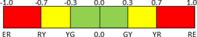

  

  Traffic light model on top of PQ-Indic

• Yellow: A slight change of the charging power is required, since the power quality of the grid is not optimal but still above or below a certain critical threshold. This change can be in form of proactive increase or decrease of the charging power. In the yellow state, the grid has high priority and requirements of the charging process can be taken into account only to a certain degree. The PQ-Indic value is within (RY,YG]∪[GY,YR), where RY=−0.7, YG=−0.3, GY=0.3 and YR=0.7.

• Red: The situation of the grid is critical and the load at the charging station must be reduced or increased according to a certain factor. The red color is defined for a PQ-Indic value within [ER,RY]∪[YR,RE], where ER=−1, RY=−0.7, YR=0.7 and RE=1.

In that regard, the six thresholds, ER_k,RY_k,YG_k,GY_k,YR_k,RE_k, for the red, yellow and green area are defined for each KPI class k separately. As a guideline, power quality standards such as EN50160 (Standard 1994) can be used. The values of K_k are translated according to a piece-wise linear interpolation function t_k(Eq. 4 and Fig. 3) to the range of [−1,1]. The PQ-Indic_k for KPI class K_k is equal to t_k(K_k).

Fig. 3

The translation function t_k(x) that translates KPI values to PQ-Indic

For simplicity we use the piece-wise linear interpolation function Eq. 4, which preserves the order of the KPI values and maps the range of different KPI classes to the same smaller range of [−1,1]. The piece-wise nature allows weighting and shifting of the range of individual KPI classes.

$$ t_{k}(x) = \left\{ \begin{array}{ll} ER & \text{if } x \in (-\infty, ER_{k}) \\ \frac{RY \cdot (ER_{k} - x) + ER \cdot (x - RY_{k})}{ER_{k} - RY_{k}} & \text{if } x \in [ER_{k}, RY_{k}] \\ \frac{YG \cdot (RY_{k} - x) + RY \cdot (x - YG_{k})}{RY_{k} - YG_{k}} & \text{if } x \in (RY_{k}, YG_{k}] \\ \frac{GY \cdot (YG_{k} - x) + YG \cdot (x - GY_{k})}{YG_{k} - GY_{k}} & \text{if } x \in (YG_{k}, GY_{k}) \\ \frac{YR \cdot (GY_{k} - x) + GY \cdot (x - YR_{k})}{GY_{k} - YR_{k}} & \text{if } x \in [GY_{k}, YR_{k}) \\ \frac{RE \cdot (YR_{k} - x) + YR \cdot (x - RE_{k})}{YR_{k} - RE_{k}} & \text{if } x \in [YR_{k}, RE_{k}] \\ RE & \text{if } x \in (RE_{k}, \infty) \\ \end{array}\right. $$

(4)

Afterwards, the different PQ-Indic_k are combined using the following criteria A₁ and A₂, which are ordered according to their importance in terms of grid stability. In this paper we focus on these two criteria because existing charging stations have the capability to mitigate overloading and voltage level by limiting the charging power. Nevertheless, this list may be extended to include additional criteria such as harmonics and frequency deviation.

• Overloading an element of the grid

  Power distribution equipment, such as transformers or cables, have an upper thermal limit which should only be exceeded for a short time. The specific thresholds can vary with the equipment type. An example that depends on the maximum allowed apparent capacity S_max is given in Table 1. In case of a transformer the values are chosen in a way, such that the transformer is operated below its maximum apparent power and optimally with highest efficiency.

  Table 1 The thresholds of KPI class from criteria A₁

• Voltage level

  Different load and generation scenarios can cause the voltage level to increase or decrease in certain areas of the low voltage distribution system. According to EN 50160 standard, this variation should be in the boundaries of ± 10% of the nominal voltage U_N during 95% of the week measured by 10-min mean RMS voltage values. As we are estimating the grid phase-by-phase, the voltage level is measured between the phase and the neutral (conductor). Generally defined thresholds for the voltage KPI class are shown in Table 2.

  Table 2 Thresholds of the voltage KPI class from criteria A₂

As the considered criteria have different priorities in terms of grid stability and the main concern of the Smart Charger is the local stability as part of the global one, the PQ-Indicator uses a 3-layer hierarchical logic to decide about the (local) grid state as depicted in Fig. 4. As highest priority, criteria A₁ represents the transformer loading. For this purpose, the translation function t_k(x) (in Eq. 4) is applied on the measured load of the transformer to calculate $PQ - Indic_{A_{1}}$. In case $PQ - Indic_{A_{1}}$ is colored red, a critical load reduction or increase is required and the PQ-indicator will ignore criteria A₂ returning $PQ - Indic_{A_{1}}$ as overall PQ-Indic of the grid. Otherwise, the PQ-Indicator will compute three more values regarding to the criteria A₂ describing the voltage in three places in the grid: $PQ - Indic_{A_{2}}^{CS}$ at the CS, $PQ - Indic_{A_{2}}^{Tran}$ at the transformer and $PQ - Indic_{A_{2}}^{Critical}$ at a critical point in the low voltage grid. In order to determine the critical point for each charging station, we identify several points with low and high voltage magnitude in the low voltage grid and choose the one which is most influenced by changes of the stations’ charging behavior.

Fig. 4

Hierarchical decision logic of the PQ-Indicator based on the traffic light model

In the second level, the PQ-Indicator will use Algorithm 1 to indicate the state of the grid regarding A₂. In case $PQ - Indic_{A_{2}}$ is colored yellow or red, this value is directly returned. Otherwise, the output is calculated by the third level taking the situation at the critical point into account. Hence, if the PQ-Indic at the critical point is colored yellow or red, $PQ - Indic_{A_{2}}^{Critical}$ is used as output of the PQ-Indicator, otherwise, the PQ-Indic at the charging station $\left (PQ - Indic_{A_{2}}^{CS}\right)$ defines the return value.

Smart Charger

According to OCPP 2.0 (Open Charge Alliance 2017), charging stations can handle different types of the charging profiles. The ChargingStationMaxProfile is usually based on a 24 h forecast from the DSO, TxProfiles are used for single charging transactions and ChargingStationExternalConstraints profile represent limits set from external systems. This different profiles are stacked and used by their prioritized stack level. The Composite Schedule combines the different profile types by calculating the minimum in each time interval. During the charging process, our smart charging algorithm controls the charging process using external profiles at a high stack level.

The smart charging algorithm starts once a vehicle is plugged into a connector. The algorithm of the Smart Charger is modeled as Finite State Machine (FSM), which stores the last PQ traffic light estimation of the gird. In order to differentiate the positive and negative PQ-Indic value of each color in the aforementioned traffic light model, we split the two states red and yellow into two states from each color. As a result there is a low-red state (light diagonal red in Fig. 5) representing the state of having a negative value of red-colored PQ-Indic, which requires a load reduction. In addition there is a high-red state (dark vertical red in Eq. 5) representing the positive value of red-colored PQ-Indic, which requires a load increase. The yellow state is split accordingly (large grid and diagonal brick in Fig. 5). Because nowadays charging stations cannot control the charging process per phase and, therefore, the design of the FSM only considers the overall charging power, we aggregate the input PQ-Indic values as follows:

$$ \underset{i\in{\{A,B,C\}}}{agg(PQ_{i})} = \left\{ \begin{array}{ll} \underset{i\in{\{A,B,C\}}}{avg(PQ_{i})} & \text{if } \forall i\in{\{A,B,C\}}\text{: } PQ_{i} \text{ is green} \\ \underset{i\in{\{A,B,C\}}}{max(PQ_{i})} & \text{else if } \forall i\in{\{A,B,C\}}\text{: } PQ_{i} \text{ is green} \\ & \quad \qquad \qquad \qquad \qquad \, \lor PQ_{i}\text{ is high-yellow} \\ & \quad \qquad \qquad \qquad \qquad \,\lor \text{} PQ_{i}\text{ is high-red}\\ \underset{i\in{\{A,B,C\}}}{min(PQ_{i})} & otherwise\\ \end{array}\right. $$

(5)

Fig. 5

FSM of the Smart Charger based on the traffic light model: For simplification within the box containing the operational states, only the outgoing and incoming transitions of the “low red” state are shown. All other states are connected similarly to each other. Furthermore, the state machine can transit from any operational states to the standby and end state

where PQ_i is the ’PQ-Indic’ value of phase i. We intend to use a conservative aggregation when phases are in different colored states since phase balancing is performed by the CS. In contrast, aggressive aggregation is used when the grid is asking for load increase on one or more phases while other states are at least green. In that case a charging increase is allowed on all phases, hence we choose the maximum in order to mitigate the biggest problem first. In the case of green states on all phases, the average perfectly reflects the situation.

Finite state machine

The FSM used within the Smart Charger is shown in Fig. 5 and its definition is described in the following section. The FSM consists of seven states that are grouped to three different types:

• Operational states: low red, low yellow, green, high yellow, and high-red state representing the different ’PQ-Indic’ color ranges.

• Standby state: The gray state models the charging state after the desired State of Charge (SoC) is reached.

• End state (blue state with horizontal lines): With maximum SoC or unplugged EV it is not longer possible to control the charging operation.

The transitions in the FSM are labeled by two parts: Event and Guard. In the proposed FSM we have three kinds of events that can trigger the state transition: Input of a new PQ-Indic value, unplugging of the vehicle and changing of the SoC of the battery. Each state transition can have a prerequisite, which is modeled by the logical condition of a guard. If the condition of a guard does not match, the FSM remains in the last state. Finally, each state transition can have an action which specifies the output of the Smart Charger. In our case, the action defines the new charging power of the ongoing charging process.

The low-red state is considered as the start state, since the charging operation will start slowly and it adapts a conservative approach concerning the grid stability. The transition to the end state occurs whenever the driver unplugs the vehicle or the battery is fully charged (equals SoC = 100). If the desired SoC_end (defined by the end user) is reached, the FSM transits to the charging standby state (gray state). Within this state the Smart Charger can react on critical grid situations using the still plugged EV, only in case the ’PQ-Indic’ value is positive red-colored, hence requires increase of charging power capacity.

Transitions and actions

In this section, the used capacity of an active charging process at charging station C_i at time t is denoted as $\mathcal {U}_{i}(t)$, the maximum capacity is written as $\mathcal {M}_{i}$ and the users’ charging profile is denoted as $\mathcal {C}_{i}(t)$. In all cases, the action of transitions, which reveals the new charging power, should not be bigger than $\mathcal {M}_{i}$. A safety upper margin is defined by μ in order to stay aligned with the users charging profile regarding the battery state of health and the charging duration. This safety margin is used as a buffer to compensate grid problems that may lead to a short reduction of charging power. Other way round, the minimum charging power needs to be set to a value $\mathcal {C}_{min}$ higher than zero to avoid disconnection of the vehicle.

The action of the transitions mainly rely on the destination state, which is equal to the color of the new input PQ-Indic value. In the following, the single transitions are given by source →destination. The source and destination can also be an asterisk.

• ∗→ low-red state

  If the new PQ-Indic value is colored low-red, the Smart Charger needs to reduce the charging power. Since this state is considered to be highly critical for the grid, the resulting action is defined in a polynomial way. We calculate δ as the percentage of change in the currently used power.

  $$ \begin{aligned} \delta &= (\mathrm{PQ\text{-}Indic} + 1)^{\alpha}\\ \mathcal{U}_{i}(t+1) &= \max\big(\delta \cdot \mathcal{U}_{i}(t), \mathcal{C}_{min}\big) \end{aligned} $$

  (6)

  The parameter α in Eq. 6 needs to be greater than 1 in order to match a polynomial decrease. Therefore, δ∈[0,0.3) because PQ-Indic∈[−1,−0.7]. As a result, in any case the decrease of the charging power is greater than 70% of the currently used charging power.

  The parameter α can be defined depending on the source of the transition or by comparing with the last PQ-Indic value.

• ∗→ (low and high)-yellow states

  Within the boundaries of the yellow-colored PQ-Indic, the gird is not stable, but it is not highly critical like in the red states. Hence, the transitions to this state can consider the users’ charging profile. The change in the charging power capacity is calculated by a linear function, which depends on the PQ-Indic value and can be parameterized by the source state of the transition.

  $$ \begin{aligned} \delta_{1} &= 1 + (\beta_{1} \cdot (\mathrm{PQ\text{-}Indic}+ YG + 0.1))\\ \delta_{2} &= 1 + (\beta_{2} \cdot (\mathrm{PQ\text{-}Indic}+ GY - 0.1)) \end{aligned} $$

  (7)
  $$ \mathcal{U}_{i}(t+1) = \left\{ \begin{array}{ll} \min\left(\delta_{1} \cdot \mathcal{U}_{i}(t), (1+2\mu) \cdot {\mathcal{C}}_{i}(t+1), \mathcal{M}_{i}\right) & \mathrm{PQ\text{-}Indic} \geq GY \\ \max\left(\delta_{2} \cdot \mathcal{U}_{i}(t), \mathcal{C}_{min}\right) & \mathrm{PQ\text{-}Indic} \leq YG\\ \end{array}\right. $$

  The parameter β₁ and β₂ in Eq. 7 are taken from $\mathbb {R}$ and can in example be configured by the source of the transition. However, in any case the new charging power is limited by the minimum of $\mathcal {C}_{min}$ and the maximum of $\mathcal {M}_{i}$.

• ∗→ green state

  Within the boundaries of the green-colored PQ-Indic, the gird is stable. In this regard, a linear increase or decrease of the currently used charging power is applied until the charging profile plus the safety margin is reached.

  $$ \begin{aligned} \lambda &= (\mathrm{PQ\text{-}Indic}+ GY + 0.1)/2\\ \delta_{1} &= \lambda \cdot (1+\mu) \cdot {\mathcal{C}}_{i}(t+1)\\ \delta_{2} &= ({\mathcal{C}}_{i}(t) - (1+\mu) \cdot {\mathcal{C}}_{i}(t+1))/2 \end{aligned} $$

  (8)
  $$\mathcal{U}_{i}(t+1) = \left\{ \begin{array}{ll} \min(\mathcal{U}_{i}(t)+ \delta_{1}, (1+\mu) \cdot {\mathcal{C}}_{i}(t+1)) & \mathcal{U}_{i}(t) \leq (1 + \mu) \cdot \mathcal{C}_{i}(t+1) \\ \mathcal{U}_{i}(t)- \delta_{2} & \mathcal{U}_{i}(t) > (1 + \mu) \cdot \mathcal{C}_{i}(t+1). \\ \end{array}\right. $$

• ∗→ high-red state

  If the new PQ-Indic value equals the high-red state, the grid is in a highly critical status and the Smart Charger must increase the charging power. Hence, a polynomial function is defined for transitions to this state.

  $$ \begin{aligned} \delta &= \omega \cdot (\mathrm{PQ\text{-}Indic})^{\varepsilon} + 1\\ \mathcal{U}_{i}(t+1)&= \min\left(\delta \cdot \mathcal{U}_{i}(t), \mathcal{M}_{i} \right) \end{aligned} $$

  (9)

  The parameters ω and ε in Eq. 10 can be defined depending on the source of the transition or by comparing with the last PQ-Indic value. The parameter ω must at least be lower than $\frac {\mathcal {M}_{i}}{\mathcal {U}_{i}(t)}$ and bigger than 1 and ε must be lower than 1 in order to match a polynomial increase. Obviously, δ is bigger than one, because ω is bigger or equal to 1 and PQ-Indic is a positive value.

• ∗→ gray state

  The gray state represents the standby phase of the charging process. In this phase, the Smart Charger only responses to highly critical grid situations by increasing the charging rate. Otherwise, the charging power is reduced continuously until it reaches $\mathcal {C}_{min}$ again in a linear way.

  $$ \begin{aligned} \delta &= \omega \cdot (\mathrm{PQ\text{-}Indic})^{\varepsilon} + 1\\ \mathcal{U}_{i}(t+1) &= \left\{ \begin{array}{ll} \min\left(\delta \cdot \mathcal{U}_{i}(t),\mathcal{M}_{i} \right) & \mathrm{PQ\text{-}Indic} \geq YR \\ \max(\mu \cdot \mathcal{U}_{i}(t), \mathcal{C}_{min}) & \mathrm{PQ\text{-}Indic} < YR\\ \end{array}\right. \end{aligned} $$

  (10)

  The parameters ε and ω in Eq. 10 are similarly defined like with transitions to the high-red state and μ∈[0,1).

Finally, oscillations between two different states (low and high red) needs to be avoided, because this affects the stability of the Smart Charger. Hence, the parameters α and ε which are used as exponential factors in the aforementioned definitions of both states, need to be different.

Evaluation

The objective of this section is to evaluate the smart charging algorithm and the reaction of EVs on control commands. The evaluation is carried out using pure (co)-simulation and PHIL. The smart charging algorithm is evaluated based on the achieved improvement of the power quality in a simulated grid. Furthermore, we compare the charging process of a simulated EV with a real and an emulated EV in order to study the reaction of EVs on the control signals from the algorithm.

Setup

For all the following evaluation scenarios, the co-simulation framework AIT Lablink is used (Faschang et al. 2013). With Lablink it is possible to replace software simulation components by different PHIL equipment in the laboratory, e.g. a hardware charging station with a Type 2 charging connector or either a real or an emulated EV based on a Resistor - Indicator - Capacitor (RLC) load model. The smart charging is carried out on the simulation of a realistic low voltage network, which is located in a small city in Bavaria. This grid connects 22 households, 21 industries, three PV systems and four charging stations to a transformer using 64 cables. The maximum distance to the transformer is given by a cable with the length of 485 meters. As power gird simulation tool we use PowerFactory (DIgSILENT 2018) from DIgSILENT. The simulation is fed with BDEW load profiles for industries, realistic load profiles for households (Tjaden et al. 2015) and real PV generation profiles. The Event-Engine is simulated by a locally installed Apache KAFKA cluster with only one node and default configuration.

The hardware charging station communicates the charging signal via a IEC 62196 Type 2 connector to the EV emulator and the real EV. This standard supports a Pulse Width Modulation (PWM) current signal, which indicates the amount of current that can be provided by the charging station. Since this value is valid for all three phase, phase-balancing is not possible with that protocol. Furthermore, only integer current values are allowed, hence the charging power capacity can only be controlled in discrete steps. The real charging station supports 3-phase charging from 6 to 32 A, resulting in a maximum charging power of 22 kW.

The grid simulator, Event-Engine, PQ-Indicators, Smart Chargers and the charging stations in Fig. 6 are implemented as LabLink clients. These clients can communicate with each other using a Message Queuing Telemetry Transport (MQTT) message bus. The KPI values from the power simulation tool are published to the Event-Engine. The PQ-Indicator subscribes the KPI values from the Event-Engine, calculates its internal equations and forwards the output to the Smart Charger, which produces a charging signal that is either sent to the real charging station hardware or to a simulated charging station. In both cases, the measured or calculated power demand of the EV is injected into the power simulation tool for the next simulation step.

Fig. 6

Evaluation Setup

The KPI thresholds for voltage and loading of the transformer are configured in the PQ-Indicator as shown in Table 3. From EN 50160 we know that in low and medium voltage networks the voltage level must be within ± 10% of the nominal voltage during 95% of the week measured by 10 min mean RMS values (Standard 1994). As the maximum allowed voltage deviation includes the medium voltage network and is constantly transmitted to the low voltage grid in case no On Load Tap Changer (OLTC) is installed, we decided to use a smaller range of ± 10 volt (which is about ± 5%) and a time interval of one minute. Due to the setup of our test grid, overloading of the transformer starts at 37.5% of the rated apparent power of the transformer, which is given by 400kVA.

Table 3 The thresholds of the overloading KPI class (first part) and the voltage KPI class (second part)

The parameters of the smart charging algorithm are configured according to Table 4. The Smart Charger needs to provide at least a minimum of 1.3 kW (6 A) in order that the EV does not disconnect and the maximum is given by the limitation of the hardware charging station. For simplicity, we configured the charging profile to be the maximum charging power for the whole charging process. The remaining parameters are chosen in a way such that the charging control signal changes smoothly and result in a reasonable reaction on the PQ-Indic.

Table 4 Parameter configuration of the smart charging algorithm

We simulate a whole working day during the winter in the realistic Bavarian grid with four charging stations equipped with our Smart Charger connected to different connection points in the grid. As depicted in Fig. 7, one charging station is located as far as possible from the transformer at the critical point of the grid in terms of voltage drop (C₂), the second charging station is located at the second main feeder line that is supplied by the transformer (C₄) and the remaining two charging stations are located near to the transformer, like it is the case in the real Bavarian grid.

Fig. 7

Schematic location of the four charging station in the tested grid

Analysis

In order to evaluate the impact of our smart charging algorithm on the power quality, we assume the worst case scenario, where EVs are connected to all charging stations and they charge for the whole simulation time period, without disconnection. Furthermore, the EVs charge with a constant load over the whole period, e.g. without the saturation phase of the battery. The result of our smart charging algorithm is compared against two baseline scenarios: (I) All charging stations are charging for the whole time period with their maximum charging power and (II) No charging station is charging at all. Our evaluation answers the following two questions:

• To which extend can our smart charging algorithm improve the voltage level in the grid using simulation?

• Is the result of the Smart Charger also valid using PHIL simulation?

First, comparing the voltage level at the critical point of our grid using the proposed smart charging algorithm against the two baseline scenarios in Fig. 8, it can be seen that even the lower bound baseline scenario, with no car charging at all, results in a voltage drop greater than 3% during the morning and evening peak at 08:00 - 12:15 and 15:45 - 19:30. As we only consider EV charging and no Vehicle-to-Grid solution, the Smart Charger cannot compensate under-voltage by discharging the EV and the charging power is reduced to the minimum at that time. During the other times, the smart charging algorithm controls the charging station and keeps the voltage level above the 3% limit. Every time when the voltage threshold is crossed, the Smart Charger sends a reduction charging control signal to the charging station and the voltage level returns to the allowed range. With the worst case baseline scenario, where all cars are charging simultaneously with maximum charging power, the voltage drop resides in a critical level for the whole day with a minimum value of 213.5 V.

Fig. 8

Voltage level at the critical point in the Bavarian grid during a whole day. The orange line and the green line represent the baseline scenarios, while the blue line shows the voltage level when all charging stations are controlled by our smart charging algorithm. The dotted red line is the lowest allowed voltage level for the algorithm

The second criteria we are taking into account is the loading of the transformer. During noon on our simulated day, the smart charging algorithm reacts on transformer overloading similar as on voltage bandwidth violations. The simulated apparent power, measured at the transformer, is shown in Fig. 9 and compared with the two baseline scenarios. With the worst case baseline scenario the transformer is overloaded 66.7% of the day, whereas the Smart Charger reduces this value to 1.4% with only short overloading periods.

Fig. 9

Apparent power at the transformer station during a whole day. The orange and green line represent the baseline scenario, while the blue line shows the apparent power when all charging stations are controlled by our smart charging algorithm

Because our charging stations are located at different points in the grid, we also take a look at the fairness between the controllers of the charging stations. Figure 10 shows the active power of all four charging stations and the overall utilization. Within the time range 00:00 - 06:30, when the voltage at the critical point is green, the charging stations at non-critical locations can charge with nearly their maximum charging power, while the charging station at the critical point is limited to a lower level. However, starting at 06:30 when the critical point is indicated with yellow or red voltage level all charging stations react and reduce their charging power accordingly, even so the voltage at the other charging stations is still in the green range.

Fig. 10

Power of charging stations. The colored lines represent the power of each single charging station and the gray line depicts the sum of their charging power. The dotted red line shows the rated maximum power of all four charging station

Furthermore, we verified our simulation results of the smart charging algorithm using PHIL. There are a number of different aspects that need to be considered when move from simulated to real charging operations. First of all, the real and emulated cars have a charging initialization phase and the battery runs into a saturation phase at high SoC (Zhang et al. 2006). In addition, environmental circumstances can influence the charging process and the minimum accepted charging current varies with the type of the car. Apart from these points, the tested real EV and the emulated EV behave quite similar to the simulated one and both follow the control signal sent from the hardware charging station via PWM signal. In Fig. 11 the saturation phase of the emulated car starts at around 22:06, while the rest of the time, the emulated car follows the simulated charging curve. The plot in Fig. 12 compares the simulated with the real EV, where only the starting phase, efficiency and reaction time differs. These results point out that in general our smart charging approach is applicable to real charging station hardware in the field.

Fig. 11

Comparison of the simulated charging signal with the reaction of an emulated car. At the end of the charging process the emulated car reaches its saturation phase and reduces its charging power gradually

Fig. 12

Comparison of a the simulated charging signal with the reaction of a real car. The tested real car follows nearly the simulated power, except from the starting phase which takes some time. Contrarily to the Fig. 11, the SoC of the tested car is low, hence, the saturation phase does not show in this figure

Conclusion and future work

In this work, a smart charging architecture based on real-time data stream for triggering events in the grid is presented. It is intended to be a scalable, decentralized architecture, and it targets the fairness among the different running charging processes as well. The traffic light model is applied to use the introduced grid flexibility to the e-mobility sector in a convenient way. The Smart Charger shows the ability to drastically increase the quality of power with regard to the voltage level and load at the transformer by controlling the active power used by the charging stations. In the future, other control strategies for voltage control can be investigated, for example power factor correction, stationary batteries and OLTC mechanism of the transformers. However, considering further factors of power quality beyond the voltage such as harmonics and unbalance of load can be seen as a promising direction even so existing hardware does not support this functionalities. Furthermore, the mathematical stability analysis of the proposed architecture is missing and placed on the top of to-do list in the future. Finally, the fairness among the charging processes should be investigated more deeply, e.g. optimizing it by a centralized component which has a global view on the grid and instructs the local Smart Charger to react in a way to improve the power quality in the grid in total.

References

Alonso, M, Amaris H, Germain J, Galan J (2014) Optimal charging scheduling of electric vehicles in smart grids by heuristic algorithms. Energies 7(4):2449–2475. https://doi.org/10.3390/en7042449.
Álvarez, JN, Knezović K, Marinelli M (2016) Analysis and comparison of voltage dependent charging strategies for single-phase electric vehicles in an unbalanced danish distribution grid In: 2016 51st International Universities Power Engineering Conference (UPEC), 1–6.. IEEE, Coimbra. https://doi.org/10.1109/UPEC.2016.8114062. Accessed on 20 Aug 2018. https://ieeexplore.ieee.org/document/8114062/.
Ardakanian, O, Rosenberg C, Keshav S (2013) Distributed control of electric vehicle charging In: Proceedings of the Fourth International Conference on Future Energy Systems. e-Energy ’13, 101–112.. ACM, New York. https://doi.org/10.1145/2487166.2487178. Accessed on 20 Aug 2018. https://doi.org/10.1145/2487166.2487178. Accessed on 20 Aug 2018. http://doi.acm.org/10.1145/2487166.2487178.
BDEW Bundesverband der Energie- und Wasserwirtschaft eV (2013) BDEW Roadmap, Realistic Steps for the Implementation of Smart Grids in Germany. Accessed on 2 Jan 2018. https://www.bdew.de/energie/bdew-roadmap-smart-grids/.
BDEW Bundesverband der Energie- und Wasserwirtschaft eV (2015) Smart Grid Traffic Light Concept. Accessed on 2 Jan 2018. https://www.bdew.de/media/documents/Stn_20150310_Smart-Grids-Traffic-Light-Concept_english.pdf.
Chung, C, Chynoweth J, Chu C, Gadh R (2014) Master-slave control scheme in electric vehicle smart charging infrastructure. Sci World J 2014. https://www.hindawi.com/journals/tswj/2014/462312/abs/.
Cortés, A, Martínez S (2016) A hierarchical algorithm for optimal plug-in electric vehicle charging with usage constraints. Automatica 68:119–131. https://doi.org/10.1016/j.automatica.2016.01.060. Accessed on 20 Aug 2018.
Deilami, S, Masoum AS, Moses PS, Masoum MAS (2011) Real-time coordination of plug-in electric vehicle charging in smart grids to minimize power losses and improve voltage profile. IEEE Trans Smart Grid 2(3):456–467. https://doi.org/10.1109/TSG.2011.2159816. Accessed on 20 Aug 2018.
Deutsch, T, Kupzog F, Einfalt A, Ghaemi S (2014) Avoiding grid congestions with traffic light approach and the flexibility operator. Challenges Implementing Act Distrib Syst Manag CIRED 1:1–4. Accessed on 20 Aug 2018.
DIgSILENT (2018) Digital Simulation and Network Calculation. Accessed on 20 Aug 2018. www.digsilent.de/en/powerfactory.html.
Fan, Z (2012) A distributed demand response algorithm and its application to phev charging in smart grids. IEEE Trans Smart Grid 3(3):1280–1290. https://doi.org/10.1109/TSG.2012.2185075. Accessed on 20 Aug 2018.
Faschang, M, Kupzog F, Mosshammer R, Einfalt A (2013) Rapid control prototyping platform for networked smart grid systems In: IECON 2013 - 39th Annual Conference of the IEEE Industrial Electronics Society, 8172–8176.. IEEE, Vienna. https://doi.org/10.1109/IECON.2013.6700500. Accessed on 20 Aug 2018. https://ieeexplore.ieee.org/document/6700500/.
Fernandez, RC, Weidlich M, Pietzuch P, Gal A (2014) Scalable stateful stream processing for smart grids In: Proceedings of the 8th ACM International Conference on Distributed Event-Based Systems - DEBS ’14, 276–281.. ACM Press, New York. https://doi.org/10.1145/2611286.2611326. Accessed on 20 Aug 2018. http://dl.acm.org/citation.cfm?doid=2611286.2611326.
Foster, JM, Trevino G, Kuss M, Caramanis MC (2013) Plug-in electric vehicle and voltage support for distributed solar: Theory and application. IEEE Syst J 7(4):881–888. https://doi.org/10.1109/JSYST.2012.2223534. Accessed on 20 Aug 2018.
Foundation, AS (2018) Apache Kafka: A Distributed Streaming Platform. Accessed on 8 Jan 2018. https://kafka.apache.org/.
Kong, F, Liu X, Sun Z, Wang Q (2016) Smart Rate Control and Demand Balancing for Electric Vehicle Charging In: 2016 ACM/IEEE 7th International Conference on Cyber-Physical Systems (ICCPS), 1–10.. IEEE, Vienna. https://doi.org/10.1109/ICCPS.2016.7479118. Accessed on 20 Aug 2018. http://ieeexplore.ieee.org/document/7479118/.
Lehfuss, F, Nöhrer M (2017) Evaluation of different control algorithm with low-level communication requirements to increase the maximum electric vehicle penetration. CIRED - Open Access Proc J 2017(1):1750–1754. https://doi.org/10.1049/oap-cired.2017.0265. Accessed on 20 Aug 2018.
Li, R, Wu Q, Oren SS (2014) Distribution locational marginal pricing for optimal electric vehicle charging management. IEEE Trans Power Syst 29(1):203–211. https://doi.org/10.1109/TPWRS.2013.2278952. Accessed on 20 Aug 2018.
Lopes, JAP, Soares FJ, Almeida PMR (2009) Identifying management procedures to deal with connection of electric vehicles in the grid In: 2009 IEEE Bucharest PowerTech, 1–8.. IEEE, Bucharest. https://doi.org/10.1109/PTC.2009.5282155. Accessed on 20 Aug 2018. https://ieeexplore.ieee.org/document/5282155/.
Longo, M, Zaninelli D, Viola F, Romano P, Miceli R, Caruso M, Pellitteri F (2016) Recharge stations: A review In: 2016 Eleventh International Conference on Ecological Vehicles and Renewable Energies (EVER), 1–8.. IEEE, Monte Carlo. https://doi.org/10.1109/EVER.2016.7476390. Accessed on 20 Aug 2018. https://ieeexplore.ieee.org/document/7476390/.
Martinenas, S, Knezović K, Marinelli M (2017) Management of power quality issues in low voltage networks using electric vehicles: Experimental validation. IEEE Trans Power Deliv 32(2):971–979. https://doi.org/10.1109/TPWRD.2016.2614582. Accessed on 20 Aug 2018.
Medved, T, Prislan B, Zupančič J, Gubina A (2016) A traffic light system for enhancing the utilization of demand response in lv distribution networks In: 2016 IEEE PES Innovative Smart Grid Technologies Conference Europe (ISGT-Europe), 1–5.. IEEE, Ljubljana. https://doi.org/10.1109/ISGTEurope.2016.7856303. Accessed on 20 Aug 2018. https://ieeexplore.ieee.org/document/7856303/.
Open Charge Alliance (2017) OCPP 2.0 Specification. https://www.openchargealliance.org/uploads/files/protected/OCPP-2.0.zip.
Pipattanasomporn, M, Kuzlu M, Rahman S (2012) An algorithm for intelligent home energy management and demand response analysis. IEEE Trans Smart Grid 3(4):2166–2173. https://doi.org/10.1109/TSG.2012.2201182. Accessed on 20 Aug 2018.
Restrepo, M, Morris J, Kazerani M, Cañizares CA (2018) Modeling and testing of a bidirectional smart charger for distribution system ev integration. IEEE Trans Smart Grid 9(1):152–162. https://doi.org/10.1109/TSG.2016.2547178. Accessed on 20 Aug 2018.
Rivera, J, Goebel C, Jacobsen H-A (2015) A distributed anytime algorithm for real-time ev charging congestion control In: Proceedings of the 2015 ACM Sixth International Conference on Future Energy Systems. e-Energy ’15, 67–76.. ACM, New York. https://doi.org/10.1145/2768510.2768544. Accessed on 20 Aug 2018. http://doi.acm.org/10.1145/2768510.2768544.
Sankaran, C (2002) Power Quality. The electric power engineering series. CRC Press, Boca Raton.
Shyam, R, Ganesh HBB, Kumar SS, Poornachandran P, Soman KP (2015) Apache spark a big data analytics platform for smart grid. Procedia Technol 21:171–178. https://doi.org/10.1016/j.protcy.2015.10.085. SMART GRID TECHNOLOGIES.
Simonov, M (2013) Event-driven communication in smart grid. IEEE Commun Lett 17(6):1061–1064. https://doi.org/10.1109/LCOMM.2013.043013.122798. Accessed on 20 Aug 2018.
Standard, EN (1994) 50160: Voltage characteristics of electricity supplied by public distribution systems. Eur Stand CLC, BTTF 68–6.
Taft, J, Martini PD (2013) Ultra-large scale control architecture In: 2013 IEEE PES Innovative Smart Grid Technologies Conference (ISGT), 1–6.. IEEE, Washington, DC. https://doi.org/10.1109/ISGT.2013.6497906. Accessed on 20 Aug 2018. https://doi.org/10.1109/ISGT.2013.6497906. Accessed on 20 Aug 2018. https://ieeexplore.ieee.org/document/6497906/.
Tanaka, T, Sekiya T, Tanaka H, Hiraki E, Okamoto M (2012) Smart charger for electric vehicles with power quality compensator on single-phase three-wire distribution feeders In: 2012 IEEE Energy Conversion Congress and Exposition (ECCE), 3075–3081.. IEEE, Raleigh. https://doi.org/10.1109/ECCE.2012.6342512. Accessed on 20th of Aug. 2018. https://ieeexplore.ieee.org/document/6342512/.
Tjaden, T, Joseph B, Quaschning V (2015) Repräsentative elektrische Lastprofile für Wohngebäude in Deutschland auf 1-sekündiger Datenbasis, 8.. HTW Berlin. https://doi.org/10.13140/RG.2.1.5112.0080.
Vahedi, H, Al-Haddad K (2016) A novel multilevel multioutput bidirectional active buck pfc rectifier. IEEE Trans Ind Electron 63(9):5442–5450. https://doi.org/10.1109/TIE.2016.2555279. Accessed on 20 Aug 2018.
Varela, J, Hatziargyriou N, Puglisi LJ, Rossi M, Abart A, Bletterie B (2017) The igreengrid project: Increasing hosting capacity in distribution grids. IEEE Power Energy Mag 15(3):30–40. https://doi.org/10.1109/MPE.2017.2662338. Accessed on 20 Aug 2018.
Yong, JY, Ramachandaramurthy VK, Tan KM, Mithulananthan N (2015) Bi-directional electric vehicle fast charging station with novel reactive power compensation for voltage regulation. Int J Electr Power Energy Syst 64:300–310. https://doi.org/10.1016/j.ijepes.2014.07.025. Accessed on 20 Aug 2018.
Zhang, SS, Xu K, Jow TR (2006) Charge and discharge characteristics of a commercial LiCoO2-based 18650 Li-ion battery. J Power Sources 160(2):1403–1409. https://doi.org/10.1016/j.jpowsour.2006.03.037. Accessed on 20 Aug 2018.
Zhong, Y, Xia M, Chiang H (2017) Electric vehicle charging station microgrid providing unified power quality conditioner support to local power distribution networks. Int Trans Electr Energy Syst 27(3):2262. https://doi.org/10.1002/etep.2262. Accessed on 20 Aug 2018.
Funding
This project has received funding from the European Union’s Horizon 2020 research and innovation programme under grant agreement No. 713864 (ELECTRIFIC). In addition, the validation and test of the proposed approach has been performed using the ERIGrid Research Infrastructure and is part of a project that has received funding from the European Union’s Horizon 2020 Research and Innovation Programme under the Grant Agreement No. 654113. The support of the European Research Infrastructure ERIGrid and its partner ’AIT Austria’ is very much appreciated.
Furthermore, Publication costs for this article were sponsored by the Smart Energy Showcases - Digital Agenda for the Energy Transition (SINTEG) programme.
Availability of data and materials
The datasets used and/or analyzed during the current study are available from the corresponding author on reasonable request.
About this supplement
This article has been published as part of Energy Informatics Volume 1 Supplement 1, 2018: Proceedings of the 7th DACH+ Conference on Energy Informatics. The full contents of the supplement are available online at https://energyinformatics.springeropen.com/articles/supplements/volume-1-supplement-1.
Author information
Authors and Affiliations
Contributions
AA and DD were responsible for proposing the architecture, carrying out simulations, and reporting on the results. They also wrote the first draft of the paper. FK and HdM provided research direction, supervision, and funding. They also helped to write the final version of the paper. All authors read and approved the final manuscript.
Corresponding author
Ethics declarations
Competing interests
The authors declare that they have no competing interests.
Publisher’s Note
Springer Nature remains neutral with regard to jurisdictional claims in published maps and institutional affiliations.
Rights and permissions
Open Access This article is distributed under the terms of the Creative Commons Attribution 4.0 International License(http://creativecommons.org/licenses/by/4.0/), which permits unrestricted use, distribution, and reproduction in any medium, provided you give appropriate credit to the original author(s) and the source, provide a link to the Creative Commons license, and indicate if changes were made.
About this article
Cite this article
Alyousef, A., Danner, D., Kupzog, F. et al. Enhancing power quality in electrical distribution systems using a smart charging architecture. Energy Inform 1 (Suppl 1), 28 (2018). https://doi.org/10.1186/s42162-018-0027-1
Published:
DOI: https://doi.org/10.1186/s42162-018-0027-1